The `adegraphics` package

The adegraphics package (Siberchicot et al. 2017) is a complete reimplementation of the graphical functionalities of the ade4 package (Dray and Dufour 2007). The package has been initially designed to improve the representation of the outputs of multivariate analyses performed with ade4 but as its graphical functionalities are very general, they can be used for other purposes.

The adegraphics package provides a flexible environment to produce, edit and manipulate graphs. We adopted an object oriented approach (a graph is an object) using S4 classes and methods and used the visualization system provided by the lattice (Sarkar 2008) and grid (Murrell 2005) packages. In adegraphics, graphs are R objects that can be edited, stored, combined, saved, removed, etc.

Note that we tried to facilitate the handling of adegraphics by ade4 users. Hence, the name of functions and parameters has been preserved in many cases. The main changes are listed in the appendix of this vignette so that it should be quite easy to use adegraphics. However, several new functionalities (graphical parameters, creation and manipulation of graphical objects, etc.) are now available and detailed in this vignette.

The adelist mailing list can be used to send questions and/or comments on adegraphics (see https://listes.univ-lyon1.fr/sympa/info/adelist)

An overview of object classes

In adegraphics, a user-level function produces a plot that is stored (and returned) as an object. The class architecture of the objects created by adegraphics functions is described in Figure 1.

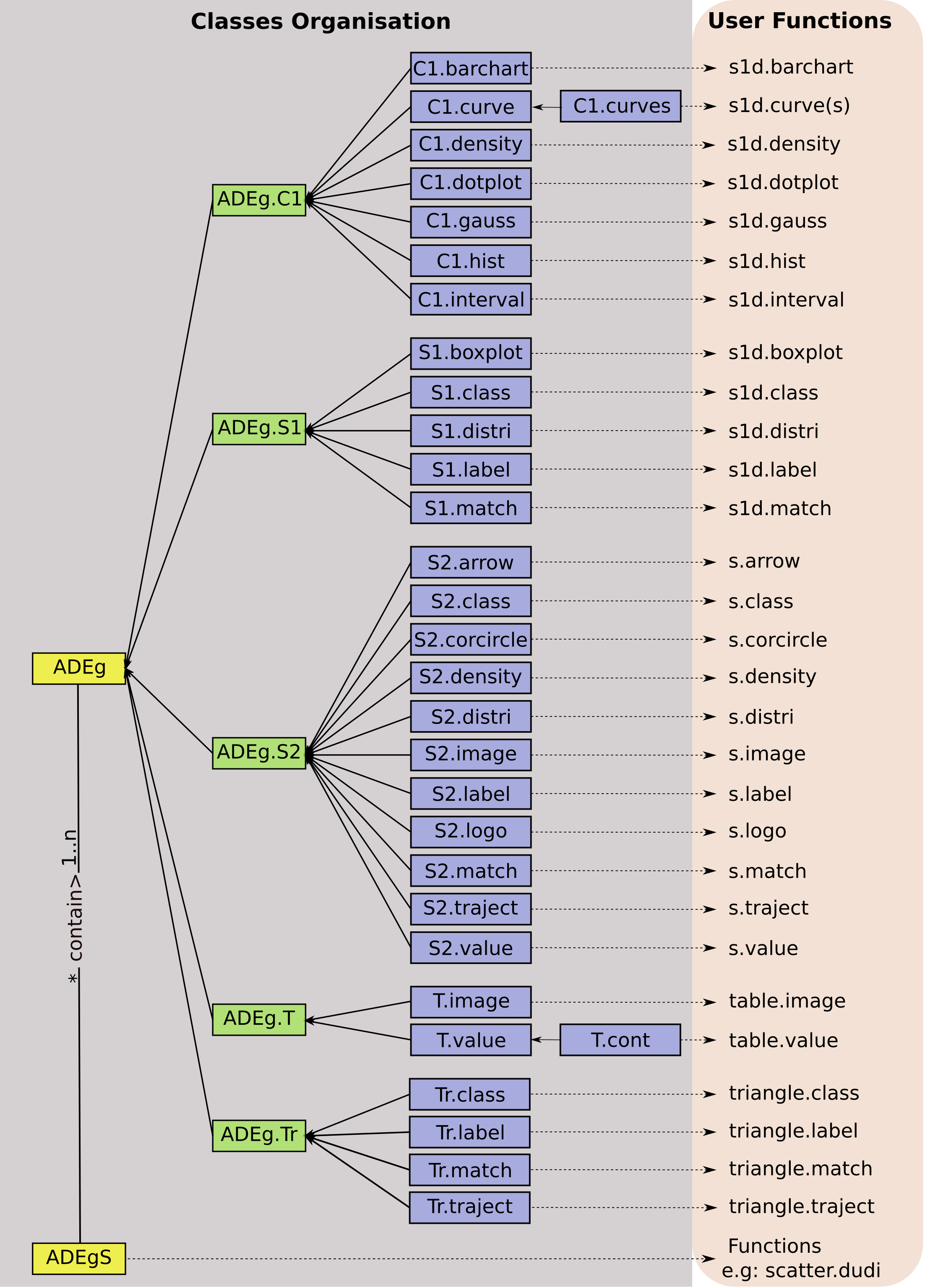
Figure 1: Classes structure and user-level functions

This class management highlights a hierarchy with two parent classes:

ADEg for simple graphs. It contains the display of a single data set using only one kind of representation (e.g., arrows, points, lines, etc.)
ADEgS for multiple graphs. It contains a collection of at least two simple graphs (ADEg, trellis or ADEgS)

The ADEg class has five child classes which are also subdivided in several child classes. Each of these five child classes is dedicated for a particular graphical data representation:

ADEg.S1: unidimensional graph of a numeric score
ADEg.S2: bidimensional graph of xy coordinates (matrix or data.frame object)
ADEg.C1: bidimensional graph of a numeric score (bar chart or curve)
ADEg.T: heat map-like representation of a data table (matrix, data.frame, dist or table object)
ADEg.Tr: ternary plot of xyz coordinates (matrix or data.frame object)

The ADEg class and its five child classes are virtual: it is not allowed to create object belonging to these classes. Users can only create objects belonging to child classes by calls to user functions (see the User functions section).

Simple graph (`ADEg` object)

In the adegraphics package, a graph is created by a call to a user function and stored as an R object. These functions allow to display the raw data but also the outputs of a multivariate analysis. The following sections describe the different graphical functions available in the package.

User functions

Several user functions are available to create a simple graph (stored as an ADEg object in R). Each function creates an object of a given class (see Figure 1). Table 1 lists the different functions, their corresponding classes and a short description. The ade4 users would not be lost: many functions have kept their names in adegraphics. The main changes are listed in Table 2.

Table 1: Graphical functions available in adegraphics

Function	Class of the returned object	Description
`s1d.barchart`	`C1.barchart`	1-D plot of a numeric score by bars
`s1d.curve`	`C1.curve`	1-D plot of a numeric score linked by curves
`s1d.curves`	`C1.curves`	1-D plot of multiple scores linked by curves
`s1d.density`	`C1.density`	1-D plot of a numeric score by density curves
`s1d.dotplot`	`C1.dotplot`	1-D plot of a numeric score by dots
`s1d.gauss`	`C1.gauss`	1-D plot of a numeric score by Gaussian curves
`s1d.hist`	`C1.hist`	1-D plot of a numeric score by bars
`s1d.interval`	`C1.interval`	1-D plot of the interval between two numeric scores
`s1d.boxplot`	`S1.boxplot`	1-D box plot of a numeric score partitioned in classes
`s1d.class`	`S1.class`	1-D plot of a numeric score partitioned in classes
`s1d.distri`	`S1.distri`	1-D plot of a numeric score by means/tandard deviations computed using an external table of weights
`s1d.label`	`S1.label`	1-D plot of a numeric score with labels
`s1d.match`	`S1.match`	1-D plot of the matching between two numeric scores
`s.arrow`	`S2.arrow`	2-D scatter plot with arrows
`s.class`	`S2.class`	2-D scatter plot with a partition in classes
`s.corcircle`	`S2.corcircle`	Correlation circle
`s.density`	`S2.density`	2-D scatter plot with kernel density estimation
`s.distri`	`S2.distri`	2-D scatter plot with means/standard deviations computed using an external table of weights
`s.image`	`S2.image`	2-D scatter plot with loess estimation of an additional numeric score
`s.label`	`S2.label`	2-D scatter plot with labels
`s.logo`	`S2.logo`	2-D scatter plot with logos (pixmap objects)
`s.match`	`S2.match`	2-D scatter plot of the matching between two sets of coordinates
`s.Spatial`	`S2.label`	Mapping of a `Spatial*` object
`s.traject`	`S2.traject`	2-D scatter plot with trajectories
`s.value`	`S2.value`	2-D scatter plot with proportional symbols
`table.image`	`T.image`	Heat map-like representation with colored cells
`table.value`	`T.value` or `T.cont`	Heat map-like representation with proportional symbols
`triangle.class`	`Tr.class`	Ternary plot with a partition in classes
`triangle.label`	`Tr.label`	Ternary plot with labels
`triangle.match`	`Tr.match`	Ternary plot of the matching between two sets of coordinates
`triangle.traject`	`Tr.match`	Ternary plot with trajectories

Table 2: Changes in functions names between ade4 and adegraphics

Function in `ade4`	Equivalence in `adegraphics`
`table.cont`, `table.dist`, `table.value`	`table.value` ¹
`table.paint`	`table.image`
`sco.boxplot`	`s1d.boxplot`
`sco.class`	`s1d.class`
`sco.distri`	`s1d.distri`
`sco.gauss`	`s1d.gauss`
`sco.label`	`s1d.label`
`sco.match`	`s1d.match`
`sco.quant`	no equivalence
`s.chull`	`s.class`²
`s.kde2d`	`s.density`
`s.match.class`	superposition of `s.match` and `s.class`
`triangle.biplot`	`triangle.match`
`triangle.plot`	`triangle.label`
`s.multinom`	`triangle.multinom`

Arguments

The list of arguments of a function are given by the args function.

library(ade4)
library(adegraphics)

## Registered S3 methods overwritten by 'adegraphics':
##   method         from
##   biplot.dudi    ade4
##   kplot.foucart  ade4
##   kplot.mcoa     ade4
##   kplot.mfa      ade4
##   kplot.pta      ade4
##   kplot.sepan    ade4
##   kplot.statis   ade4
##   scatter.coa    ade4
##   scatter.dudi   ade4
##   scatter.nipals ade4
##   scatter.pco    ade4
##   score.acm      ade4
##   score.mix      ade4
##   score.pca      ade4
##   screeplot.dudi ade4

## 
## Attaching package: 'adegraphics'

## The following objects are masked from 'package:ade4':
## 
##     kplotsepan.coa, s.arrow, s.class, s.corcircle, s.distri, s.image,
##     s.label, s.logo, s.match, s.traject, s.value, table.value,
##     triangle.class

args(s.label)

## function (dfxy, labels = rownames(dfxy), xax = 1, yax = 2, facets = NULL, 
##     plot = TRUE, storeData = TRUE, add = FALSE, pos = -1, ...) 
## NULL

Some arguments are very general and present in all user functions:

plot: a logical value indicating if the graph should be displayed
storeData: a logical value indicating if the data should be stored in the returned object. If FALSE, only the names of the data are stored. This allows to reduce the size of the returned object but it implies that the data should not be modified in the environment to plot again the graph.
add: a logical value indicating if the graph should be superposed on the graph already displayed in the current device (it replaces the argument add.plot in ade4).
pos: an integer indicating the position of the environment where the data are stored, relative to the environment where the function is called. Useful only if storeData is FALSE.
…: additional graphical parameters (see below)

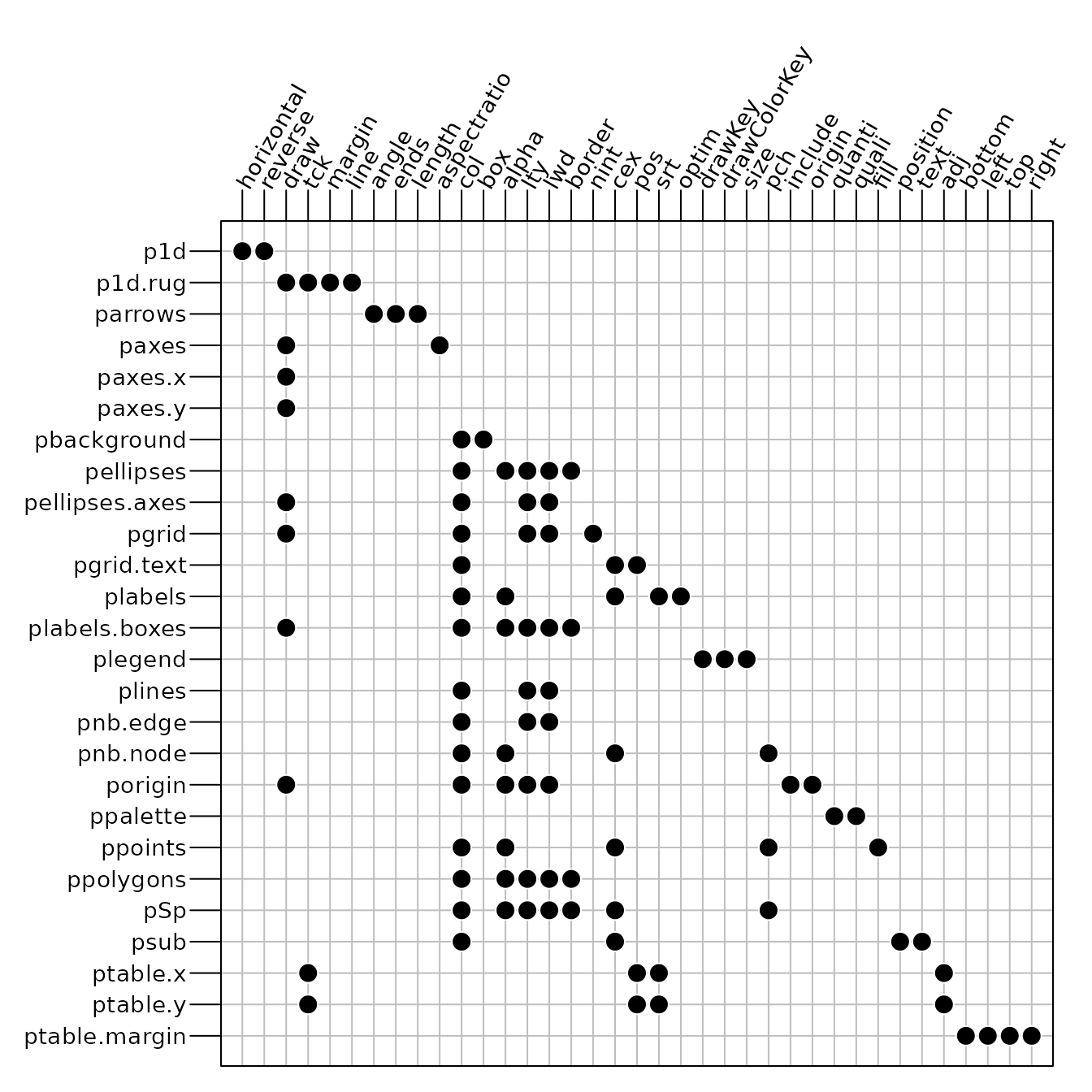
Some other arguments influence the graphical outputs and they are thus specific to the type of produced graph. Figure 2 summarizes some of these graphical parameters available for the different functions. We only reported the parameters stored in the g.args slot of the returned object (see the Parameters in g.args section).

Figure 2: Specific arguments in each object class

The ade4 users would note that the names of some arguments have been modified in adegraphics. The Appendix gives a full list of these modifications.

Slots and Methods

A call to a graphical function (see the User functions section) returns an ADEg object. Each object is defined by a number of slots and several methods are associated to this class. Let us consider the olympic data set available in the ade4 package. A principal component analysis (PCA) is applied on the olympic$tab table that contains the results for 33 participating athletes at the 1988 summer olympic games:

data(olympic)
pca1 <- dudi.pca(olympic$tab, scannf = FALSE)

The barplot of eigenvalues is then drawn and stored in g1:

g1 <- s1d.barchart(pca1$eig, p1d.horizontal = F, ppolygons.col = "white")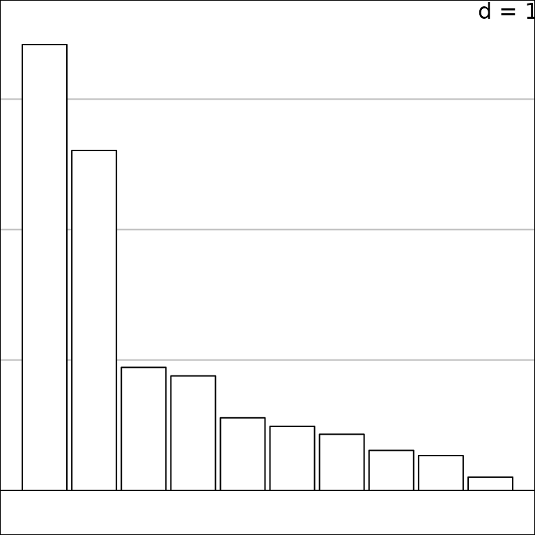

The class of the g1 object is C1.barchart which extends the ADEg class:

class(g1)

## [1] "C1.barchart"
## attr(,"package")
## [1] "adegraphics"

showClass("C1.barchart")

## Class "C1.barchart" [package "adegraphics"]
## 
## Slots:
##                                                                        
## Name:          data  trellis.par     adeg.par lattice.call       g.args
## Class:         list         list         list         list         list
##                                              
## Name:         stats       s.misc         Call
## Class:         list         list         call
## 
## Extends: 
## Class "ADEg.C1", directly
## Class "ADEg", by class "ADEg.C1", distance 2
## Class "ADEgORtrellis", by class "ADEg.C1", distance 3
## Class "ADEgORADEgSORtrellis", by class "ADEg.C1", distance 3

This object contains different slots:

slotNames(g1)

## [1] "data"         "trellis.par"  "adeg.par"     "lattice.call" "g.args"      
## [6] "stats"        "s.misc"       "Call"

These slots are defined for each ADEg object and contain different types of information. The package adegraphics uses the capabilities of the lattice package to display a graph (by generating a trellis object). Hence, several slots contain information that will be passed in the call to the lattice functions:

data: a list containing information about the data.
trellis.par: a list of graphical parameters that are directly passed to the lattice functions using the par.settings argument (see the Parameters in trellis.par section).
adeg.par: a list of graphical parameters defined in adegraphics. The list of parameters can be obtained using the adegpar function (see the Parameters in adeg.par section).
lattice.call: a list of two elements containing the information required to create the trellis object: graphictype (the name of the lattice functions that should be used) and arguments (the list of parameter values required to obtain the trellis object).
g.args: a list containing at least the different values of the graphical arguments described in Figure 2 (see the Parameters in g.args section).
stats: a list of internal preliminary computations performed to display the graph.
s.misc: a list of other internal parameters.
Call: an object of class call containing the matched call.

These different slots can be extracted using the @ operator:

g1@data

## $score
##  [1] 3.4182381 2.6063931 0.9432964 0.8780212 0.5566267 0.4912275 0.4305952
##  [8] 0.3067981 0.2669494 0.1018542
## 
## $at
##  [1]  1  2  3  4  5  6  7  8  9 10
## 
## $frame
## [1] 39
## 
## $storeData
## [1] TRUE

All these slots are automatically filled during the object creation. The trellis.par, adeg.par and g.args can also be modified a posteriori using the update method (see the Customizing a graph section). This allows to customize graphs after their creation.

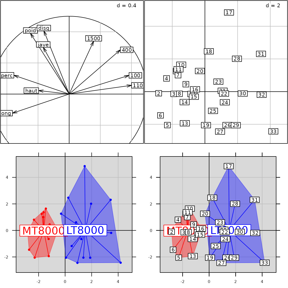
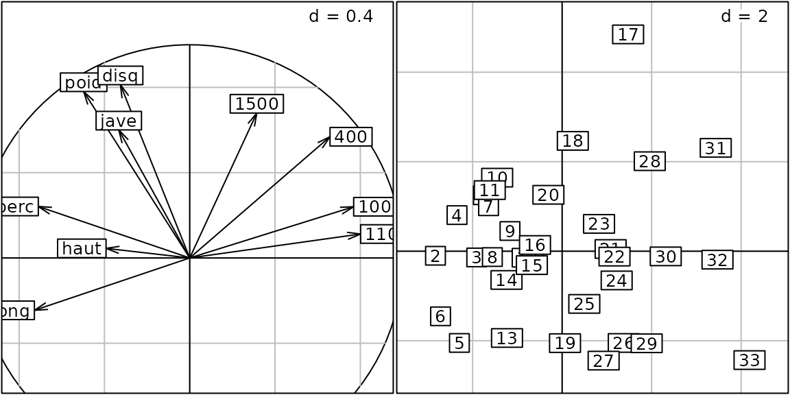
We consider the correlation circle that depicts the correlation between PCA axes and the results for each event:

g2 <- s.corcircle(pca1$co)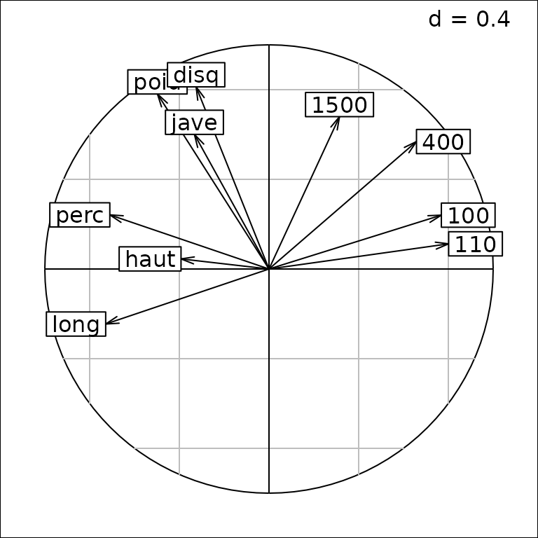

class(g2)

## [1] "S2.corcircle"
## attr(,"package")
## [1] "adegraphics"

g2@g.args

## $fullcircle
## [1] TRUE
## 
## $xlim
## [1] -1.2  1.2
## 
## $ylim
## [1] -1.2  1.2
## 
## $scales
## $scales$draw
## [1] FALSE

The argument fullcircle can be updated a posteriori so that the original object is modified:

update(g2, fullcircle = FALSE)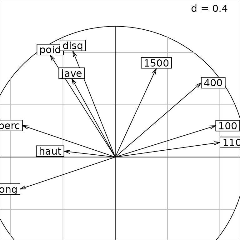

g2@g.args

## $fullcircle
## [1] FALSE
## 
## $xlim
## [1] -0.8815395  0.9544397
## 
## $ylim
## [1] -0.6344523  1.2015270
## 
## $scales
## $scales$draw
## [1] FALSE

Several other methods have been defined for the ADEg class allowing to extract information, modify or combine objects:

getcall, getlatticecall and getstats: these accessor methods return respectively the Call, the lattice.call and the stats slots.
getparameters: this method returns the trellis.par and/or the adeg.par slots.
show, print and plot: these methods display the ADEg object in the current device or in a new one.
gettrellis: this method returns the ADEg object as a trellis object. It can then be exploited using the lattice and latticeExtra packages.
superpose, + and add.ADEg: these methods superpose two ADEg graphs. It returns a multiple graph object of class ADEgS (see the The basic methods for superposition, juxtaposition and insertion section).
insert: this method inserts an ADEg graph in an existing one or in the current device. It returns an ADEgS object (see the The basic methods for superposition, juxtaposition and insertion section).
cbindADEg, rbindADEg: these methods combine several ADEg graphs. It returns an ADEgS object (see the The basic methods for superposition, juxtaposition and insertion section).
update: this method modifies the graphical parameters after the ADEg creation. It updates the current display and returns the modified ADEg (see the Customizing a graph section).

For instance:

getcall(g1) ## equivalent to g1@Call

## s1d.barchart(score = pca1$eig, p1d.horizontal = F, ppolygons.col = "white")

A biplot-like graph can be obtained using the superpose method. The result is a multiple graph:

g3 <- s.label(pca1$li)
g4 <- s.arrow(5 * pca1$c1, add = TRUE)

class(g4)

## [1] "ADEgS"
## attr(,"package")
## [1] "adegraphics"

In addition, some object classes have specific methods. For instance, a zoom method is available for ADEg.S1 and ADEg.S2 classes. For the ADEg.S2 class, the method addhist (see the The basic methods for superposition, juxtaposition and insertion section) decorates a 2-D graph by adding marginal distributions as histograms and density lines (this method replaces and extends the s.hist function of ade4).

zoom(g3, zoom = 2, center = c(2, -2))

Multiple graph (`ADEgS` object)

The adegraphics package provides class ADEgS to manage easily the combination of several graphs. This class allows to deal with the superposition, insertion or juxtaposition of several graphs in a single object. An object of this class is a list containing several graphical objects and information about their positioning. Different ways to generate ADEgS objects are described below.

Slots and Methods

The class ADEgS is used to store multiple graphs. Different slots are associated to this class (use the symbol @ to extract information):

ADEglist: a list of graphs stored as trellis, ADEg and/or ADEgS objects.
positions: a matrix containing the positions of the graphs. It has four columns and as many rows as the number of graphical objects in the ADEglist slot. For each graph (i.e. row), it contains the coordinates of the bottom-left and top-right corners in npc units (i.e. normalized parent coordinates varying between 0 and 1).
add: a square binary matrix with as many rows and columns as the number of graphical objects in the ADEglist slot. It allows to manage the superposition of graphs: the value at the i-th row and j-th column is equal to 1 if the j-th graphical object is superposed on the i-th. Otherwise, this value is equal to 0.
Call: an object of class call containing the matched call.

Several methods have been implemented to obtain information, edit or modify ADEgS objects. Several methods are inspired from the management of list in R:

[, [[ and $: these methods extract one or more elements from the ADEgS object.
getpositions, getgraphics and getcall: these methods return the positions, the ADEglist and the Call slots, respectively.
names and length: these methods return the names and number of graphs contained in the object.
[[<- and names<-: these methods replace a graph or its name in an ADEgS object (acts on the ADEglist slot).
show, plot and print: these methods display the ADEgS object in the current device or in a new one.
superpose and +: these methods superpose two graphs. It returns a multiple graph object of class ADEgS (see the The basic methods for superposition, juxtaposition and insertion section).
insert: this method inserts a graph in an existing one or in the current device. It returns a multiple graph object of class ADEgS (see the The basic methods for superposition, juxtaposition and insertion section).
cbindADEg, rbindADEg: these methods combine several graphs. It returns an ADEgS object (see the The basic methods for superposition, juxtaposition and insertion section).
update: this method modifies the names and/or the positions of the graphs contained in an ADEgS object. It updates the current display and returns the modified ADEgS.

We will show in the next sections how these methods can be used to deal with ADEgS objects.

Creating an `ADEgS` object by hand

The ADEgS objects can be created by easy manipulation of several simple graphs. Some methods (e.g., insert, superpose) can be used to create a compilation of graphs by hand.

The basic methods for superposition, juxtaposition and insertion

The functions superpose, + and add.ADEg allow the superposition of an ADEg/ADEgS object on an ADEg/ADEgS object.

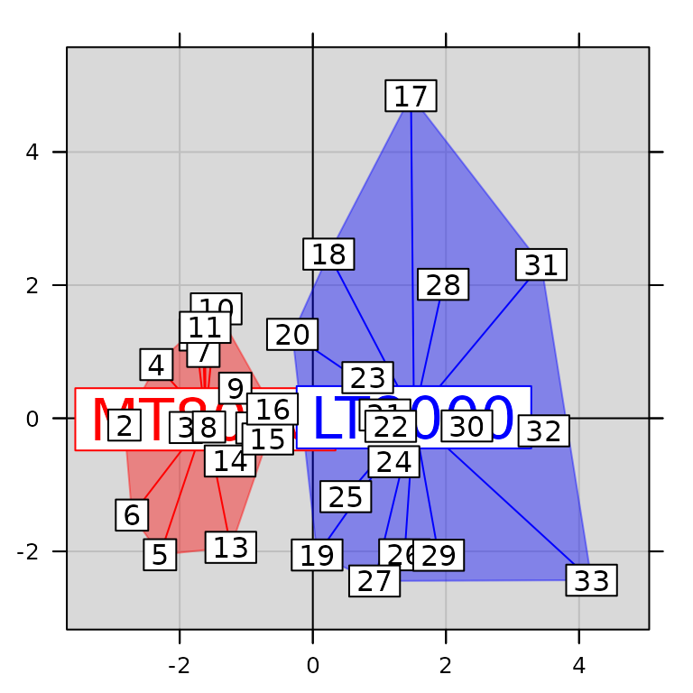
The vector olympic$score contains the total number of points computed for each participant. This vector is used to generate a factor partitioning the participants in two groups according to their final result (more or less than 8000 points):

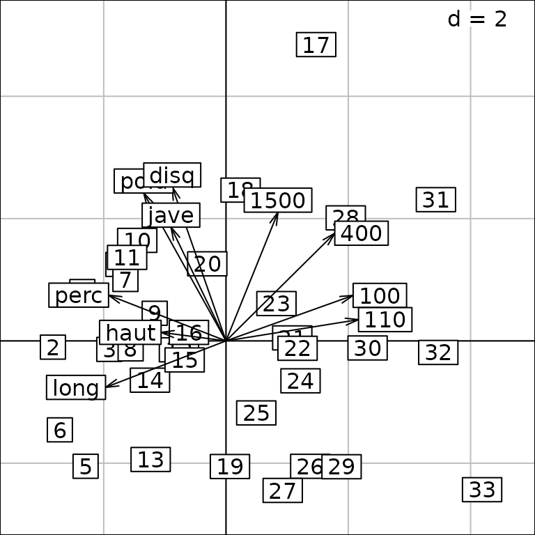
fac.score <- factor(olympic$score < 8000, labels = c("MT8000", "LT8000"))

These two groups can be represented on the PCA factorial map using the s.class function:

g5 <- s.class(pca1$li, fac.score, col = c("red", "blue"), chullSize = 1, ellipseSize = 0, 
              plabels.cex = 2, pbackground.col = "grey85", paxes.draw = TRUE)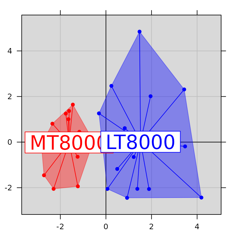

The graph with the labels (object g3) can then be superposed on this one:

g6 <- superpose(g5, g3, plot = TRUE) ## equivalent to g5 + g3

class(g6)

## [1] "ADEgS"
## attr(,"package")
## [1] "adegraphics"

In the case of a superposition, the graphical parameters (e.g., background and limits) of the first graph (the one below) are used as a reference and applied to the second one (the one above). Note that it is also possible to use the add = TRUE argument in the call of a simple user function (functions described in Table 1) to perform a superposition. The graph g6 can also be obtained by:

g5
s.label(pca1$li, add = TRUE)

The functions cbindADEg and rbindADEg allows to combine several graphical objects (ADEg, ADEgS or trellis) by rows or by columns. The new created ADEgS contains the list of the reduced graphs:

rbindADEg(cbindADEg(g2, g3), cbindADEg(g5, g6), plot = TRUE)

The function insert allows the insertion of a graphical object on another one (ADEg or ADEgS). It takes the position of the inserted graph as an argument:

g7 <- insert(g2, g6, posi = c(0.65, 0.65, 0.95, 0.95))

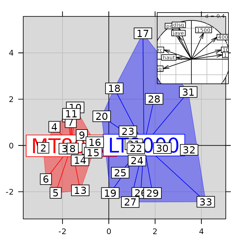
class(g7)

## [1] "ADEgS"
## attr(,"package")
## [1] "adegraphics"

The different methods associated to the ADEgS class allow to obtain information and to modify the multiple graph:

length(g7)

## [1] 3

names(g7)

## [1] "g1" "g2" "X"

names(g7) <- c("chulls", "labels", "cor")
class(g7[1])

## [1] "ADEgS"
## attr(,"package")
## [1] "adegraphics"

class(g7[[1]])

## [1] "S2.class"
## attr(,"package")
## [1] "adegraphics"

class(g7$chulls)

## [1] "S2.class"
## attr(,"package")
## [1] "adegraphics"

The multiple graph contains three simple graphs. It can be easily updated. For instance, the size of the inserted graph can be modified:

pos.mat <- getpositions(g7)
pos.mat

##           [,1] [,2] [,3] [,4]
##           0.00 0.00 1.00 1.00
##           0.00 0.00 1.00 1.00
## positions 0.65 0.65 0.95 0.95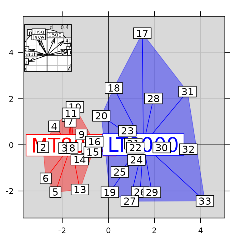

pos.mat[3,] <- c(0.1, 0.7, 0.3, 0.9)
update(g7, positions = pos.mat)

The graphs themselves can be modified, without affecting the global structure of the ADEgS object. Here, we replace the correlation circle by the barplot of eigenvalues:

g7[[3]] <- g1
g7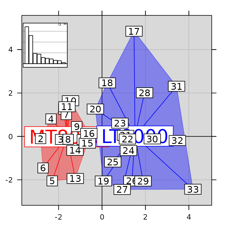

The addhist method adds univariate marginal distributions around an ADEg.S2 and returns an ADEgS object:

addhist(g3)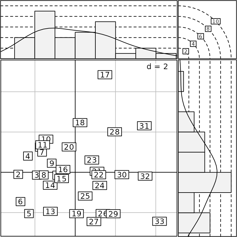

More examples are available in the help page by typing example(superpose), example(insert), example(add.ADEg) and example(addhist) in the R session.

The `ADEgS` function

The ADEgS function provides the most elementary and flexible way to create an ADEgS object. The different arguments of the function are:

adeglist: a list of several trellis, ADEg and/or ADEgS objects.
positions: a matrix with four columns and as many rows as the number of graphical objects in the ADEglist slot. For each subgraph, i.e. in each row, the coordinates of the top-right and the bottom-left hand corners are given in npc units (i.e., normalized parent coordinates varying from 0 to 1).
layout: an alternative way to specify the positions of graphs. It could be a vector of length 2 indicating the number of rows and columns used to split the device (similar to mfrow parameter in basic graphs). It could also be a matrix specifying the location of the graphs: each value in this matrix should be 0 or a positive integer (similar to layout function for basic graphs).
add: a square matrix with as many rows and columns as the number of graphical objects in the ADEglist slot. The value at the i-th row and j-th column is equal to 1 if the j-th graphical object is superposed to i-th one. Otherwise, this value is equal to 0.
plot: a logical value indicating if the graphs should be displayed.

When users fill only one argument among positions, layout and add, the other values are automatically computed to define the ADEgS object.

We illustrate the different possibilities to create objects with the ADEgS function. Simple juxtaposition using a vector as layout:

ADEgS(adeglist = list(g2, g3), layout = c(1, 2))

Layout specified as a matrix:

mlay <- matrix(c(1, 1, 0, 1, 1, 0, 0, 0, 2), byrow = T, nrow = 3)
mlay

##      [,1] [,2] [,3]
## [1,]    1    1    0
## [2,]    1    1    0
## [3,]    0    0    2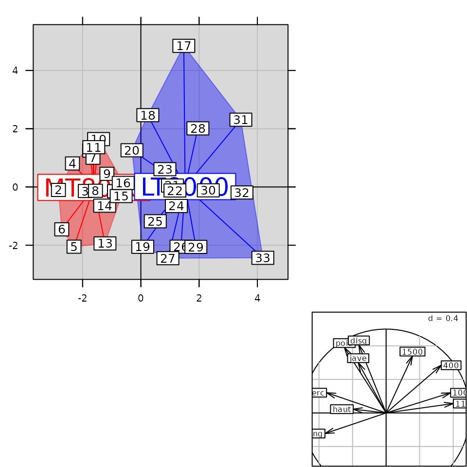

ADEgS(adeglist = list(g6, g2), layout = mlay)

Using the matrix of positions offers a very flexible way to arrange the different graphs:

mpos <- rbind(c(0, 0.3, 0.7, 1), c(0.5, 0, 1, 0.5))
ADEgS(adeglist = list(g3, g5), positions = mpos)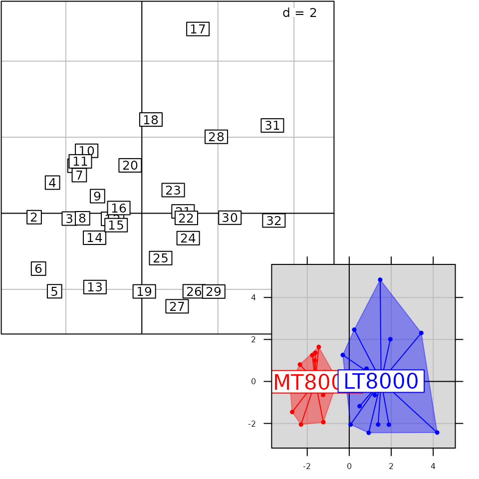

Lastly, superposition can also be specified using the add argument:

ADEgS(list(g5, g3), add = matrix(c(0, 1, 0, 0), byrow = TRUE, ncol = 2))

More examples are available in the help page by typing example(ADEgS) in the R session.

Automatic collections

The package adegraphics contains functionalities to create collections of graphs. These collections are based on a simple graph repeated for different groups of individuals, variables or axes. The building process of these collections is quite simple (definition of arguments in the call of a user function) and leads to the creation of an ADEgS object.

Partitioning the data (`facets`)

The adegraphics package allows to split up the data by one variable (factor) and to plot the subsets of data together. This possibility of conditional plot is available for all user functions (except the table.* functions) by setting the facets argument. This is directly inspired by the functionalities offered in the lattice and ggplot2 packages.

Let us consider the jv73 data set. The table jv73$morpho contains the measures of 6 variables describing the geomorphology of 92 sites. A PCA can be performed on this data set:

data(jv73)
pca2 <- dudi.pca(jv73$morpho, scannf = FALSE)
s.label(pca2$li)

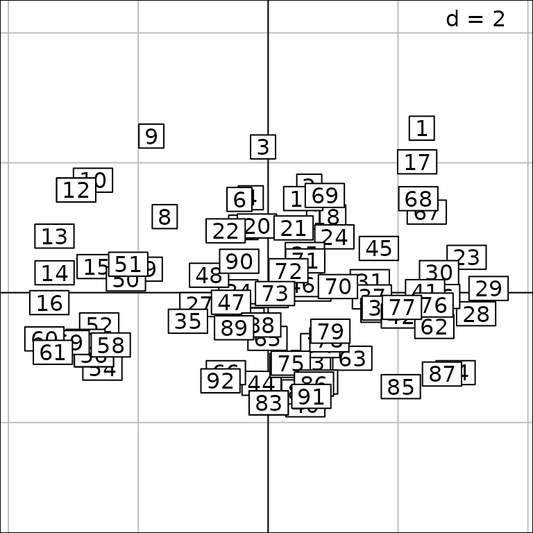
The sites are located on 12 rivers (jv73$fac.riv) and it is possible to represent the PCA scores for each river using the facets argument:

g8 <- s.label(pca2$li, facets = jv73$fac.riv)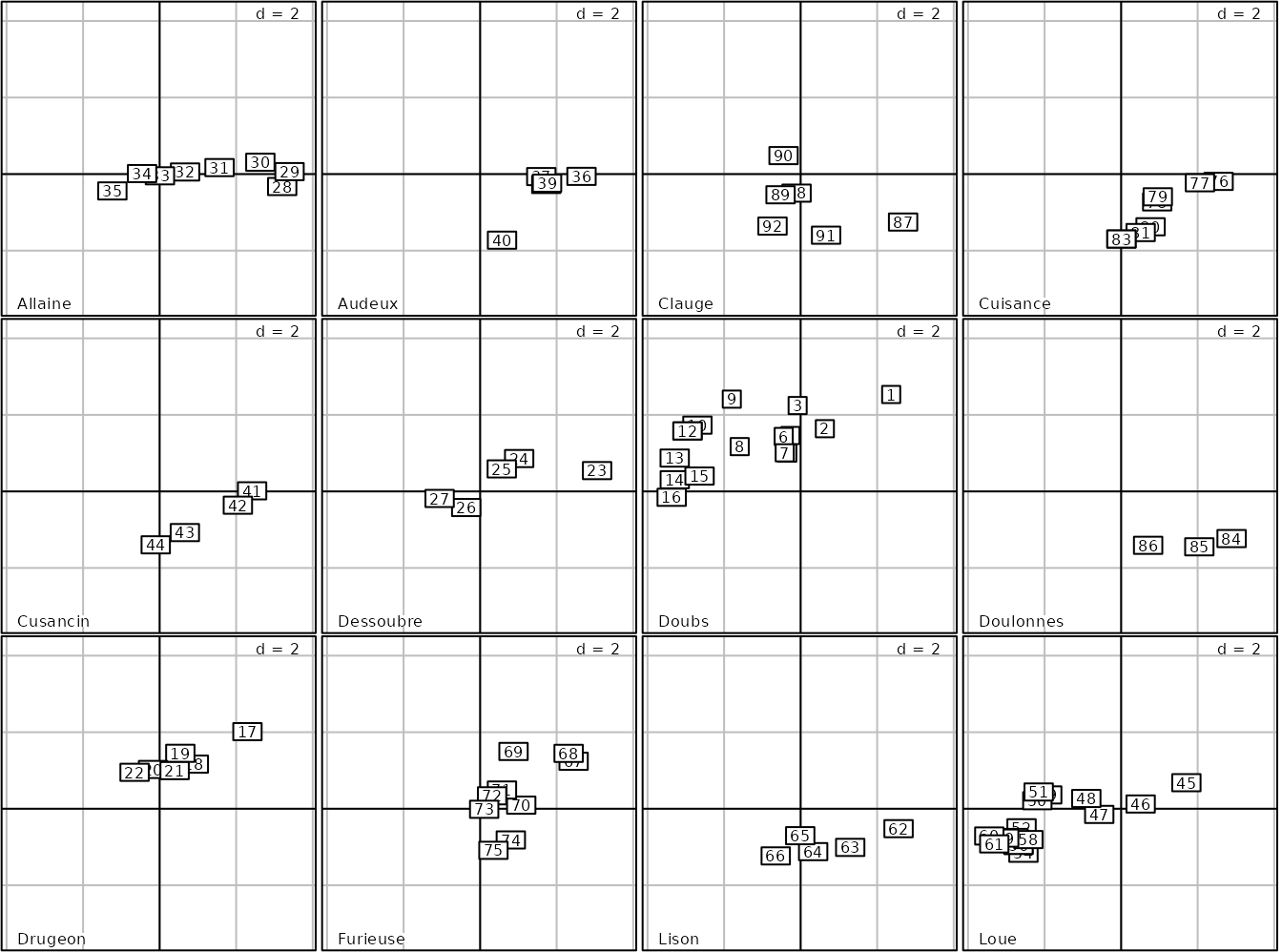

length(g8)

## [1] 12

names(g8)

##  [1] "Allaine"   "Audeux"    "Clauge"    "Cuisance"  "Cusancin"  "Dessoubre"
##  [7] "Doubs"     "Doulonnes" "Drugeon"   "Furieuse"  "Lison"     "Loue"

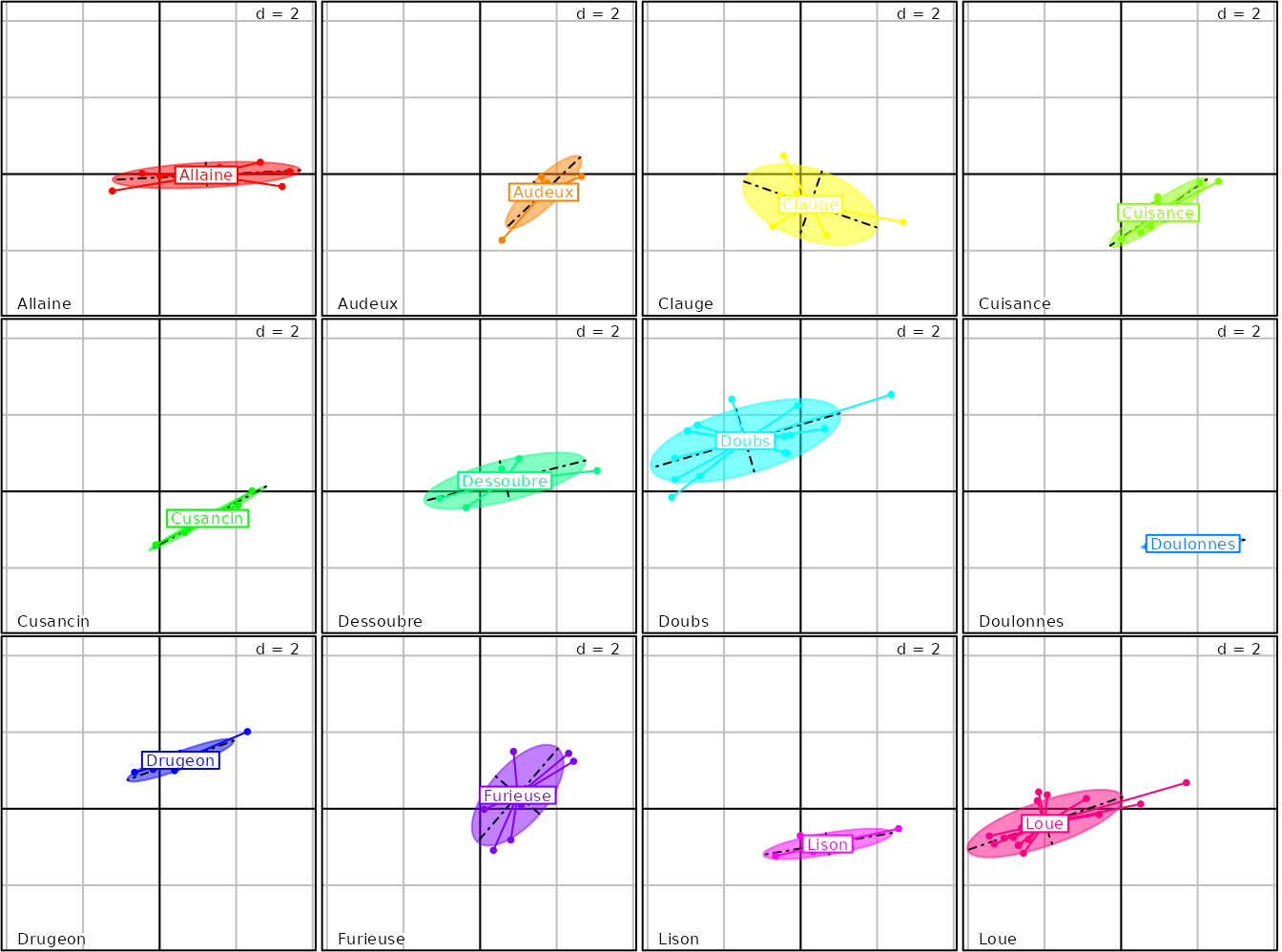
The ADEgS returned object contains the 12 plots. It is then possible to focus on a given river (e.g., the Doubs river) by considering only a subplot (e.g., type g8$Doubs). The facets functionality is very general and available for the majority of adegraphics functions. For instance, with the s.class function:

s.class(pca2$li, fac = jv73$fac.riv, col = rainbow(12), facets = jv73$fac.riv)

Multiple axes

All 2-D functions (i.e. s.*) returning an object inheriting from the ADEg.S2 class have the xax et yax arguments. These arguments allow to choose which column of the main argument (i.e. df) should be plotted as x and y axes. As in ade4, these two arguments can be simple integers. In adegraphics, the user can also specify vectors as xax and/or yax arguments to obtain multiple graphs. Here, we represent the different correlation circles associated to the first four PCA axes of the olympic data set:

pca1 <- dudi.pca(olympic$tab, scannf = FALSE, nf = 4)
g9 <- s.corcircle(pca1$co, xax = 1:2, yax = 3:4)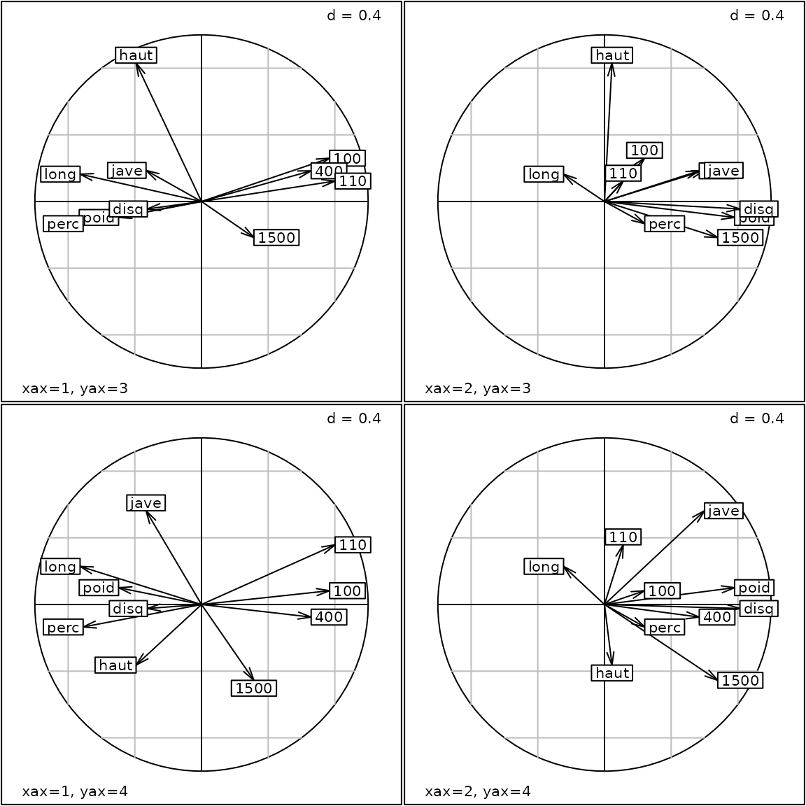

length(g9)

## [1] 4

names(g9)

## [1] "x1y3" "x2y3" "x1y4" "x2y4"

g9@positions

##      [,1] [,2] [,3] [,4]
## [1,]  0.0  0.5  0.5  1.0
## [2,]  0.5  0.5  1.0  1.0
## [3,]  0.0  0.0  0.5  0.5
## [4,]  0.5  0.0  1.0  0.5

Multiple score

All 1-D functions (i.e. s1d.*) returning an object inheriting from the ADEg.C1 or ADEg.S1 classes have the score argument. Usually, this argument should be a numeric vector but it is also possible to consider an object with several columns (data.frame or matrix). In this case, an ADEgS object is returned in which one graph by column is created. For instance for the olympic data set, we can represent the link between the global performance (fac.score) and the PCA scores on the first four axes (pca1$li):

dim(pca1$li)

## [1] 33  4

s1d.boxplot(pca1$li, fac.score, col = c("red", "blue"), 
  psub = list(position = "topleft", cex = 2))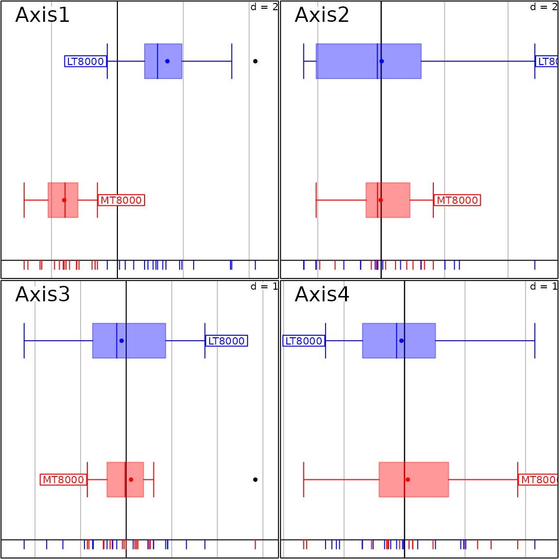

Multiple variable

Some user functions (s1d.density, s1d.gauss, s1d.boxplot, s1d.class, s.class, s.image, s.traject, s.value, triangle.class) have an argument named fac or z. This argument can have several columns (data.frame or matrix) so that each column is used to create a separate graph. For instance, we can represent the distribution of the 6 environmental variables on the PCA factorial map of the jv73$tab data set:

s.value(pca2$li, pca2$tab, symbol = "circle")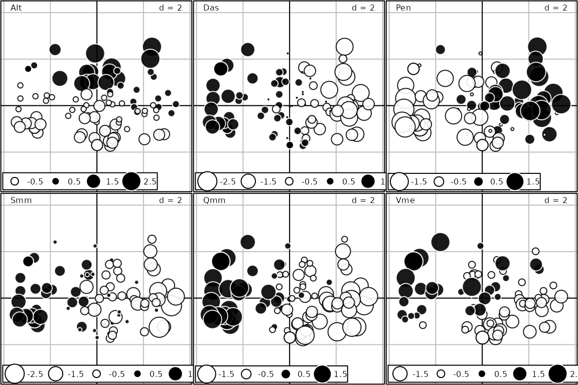

Outputs of the `ade4` package

Lastly, we reimplemented all the graphical functions of the ade4 package designed to represent the outputs of a multivariate analysis. The functions ade4::plot.*, ade4::kplot.*, ade4::scatter.* and ade4::score.* return ADEgS objects. It is now very easy to represent or modify these graphical outputs:

data(meaudret)
pca3 <- dudi.pca(meaudret$env, scannf = FALSE)
pca4 <- dudi.pca(meaudret$spe, scale = FALSE, scannf = FALSE)
coi1 <- coinertia(pca3, pca4, scannf = FALSE, nf = 3)
g10 <- plot(coi1)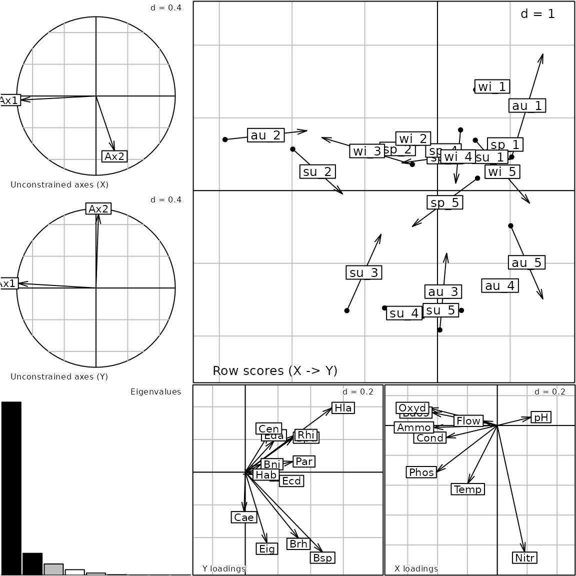

class(g10)

## [1] "ADEgS"
## attr(,"package")
## [1] "adegraphics"

names(g10)

## [1] "Xax"       "Yax"       "eig"       "XYmatch"   "Yloadings" "Xloadings"

g10@Call

## plot.coinertia(x = coi1)

Customizing a graph

Compared to the ade4 package, the main advantage of adegraphics concerns the numerous possibilities to customize a graph using several graphical parameters. These parameters are stored in slots trellis.par, adeg.par and g.args (see the Slots and Methods section) of an ADEg object. These parameters can be defined during the creation of a graph or updated a posteriori (using the update method).

Parameters in `trellis.par`

The trellis.par slot is a list of parameters that are directly included in the call of functions of the lattice package. The name of parameters and their default value are given by the trellis.par.get function of lattice.

library(lattice)
sort(names(trellis.par.get()))

##  [1] "add.line"          "add.text"          "as.table"         
##  [4] "axis.components"   "axis.line"         "axis.text"        
##  [7] "background"        "box.3d"            "box.dot"          
## [10] "box.rectangle"     "box.umbrella"      "clip"             
## [13] "dot.line"          "dot.symbol"        "fontsize"         
## [16] "grid.pars"         "layout.heights"    "layout.widths"    
## [19] "panel.background"  "par.main.text"     "par.sub.text"     
## [22] "par.title.text"    "par.xlab.text"     "par.ylab.text"    
## [25] "par.zlab.text"     "plot.line"         "plot.polygon"     
## [28] "plot.symbol"       "reference.line"    "regions"          
## [31] "shade.colors"      "strip.background"  "strip.border"     
## [34] "strip.shingle"     "superpose.line"    "superpose.polygon"
## [37] "superpose.symbol"

Hence, modifications of some of these parameters will modify the graphical display of an ADEg object. For instance, margins are defined using layout.widths and layout.heights parameters, clip parameter allows to overpass panel boundaries and axis.line and axis.text allow to customize lines and text of axes.

d <- scale(olympic$tab)
g11 <- table.image(d, plot = FALSE)
g12 <- table.image(d, axis.line = list(col = "blue"), axis.text = list(col = "red"), 
  plot = FALSE)
ADEgS(c(g11, g12), layout = c(1, 2))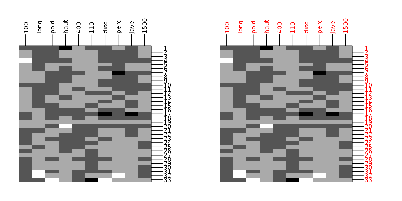

Parameters in `adeg.par`

The adeg.par slot is a list of graphical parameters specific to the adegraphics package. The name of parameters and their default value are available using the adegpar function which is inspired by the par function of the graphics package.

names(adegpar())

##  [1] "p1d"         "parrows"     "paxes"       "pbackground" "pellipses"  
##  [6] "pgrid"       "plabels"     "plegend"     "plines"      "pnb"        
## [11] "porigin"     "ppalette"    "ppoints"     "ppolygons"   "pSp"        
## [16] "psub"        "ptable"

A description of these parameters is available in the help page of the function (?adegpar). Note that each adeg.par parameter starts by the letter ’p’ and its name relates to the type of graphical element considered (ptable is for tables display, ppoints for points, parrows for arrows, etc). Each element of this list can contain one or more sublists. Details on a sublist are obtained using its name either as a parameter of the adegpar function or after the $ symbol. For example, if we want to know the different parameters to manage the display of points:

adegpar("ppoints")

## $ppoints
## $ppoints$alpha
## [1] 1
## 
## $ppoints$cex
## [1] 1
## 
## $ppoints$col
## [1] "black"
## 
## $ppoints$pch
## [1] 20
## 
## $ppoints$fill
## [1] "black"

adegpar()$ppoints

## $alpha
## [1] 1
## 
## $cex
## [1] 1
## 
## $col
## [1] "black"
## 
## $pch
## [1] 20
## 
## $fill
## [1] "black"

The full list of available parameters is summarized in Figure 3.

Figure 3: Parameters that can be set with the adegpar function.

The ordinate represents the different sublists and the abscissa gives the name of the parameters available in each sublist. Note that some row names have two keys separated by a dot: the first key indicates the first level of the sublist, etc. For example plabels.boxes is the sublist boxes of the sublist plabels. The parameters border,col, alpha, lwd, lty and draw in plabels.boxes allow to control the aspect of the boxes around labels.

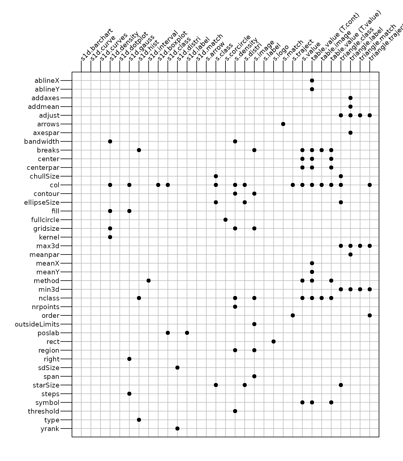
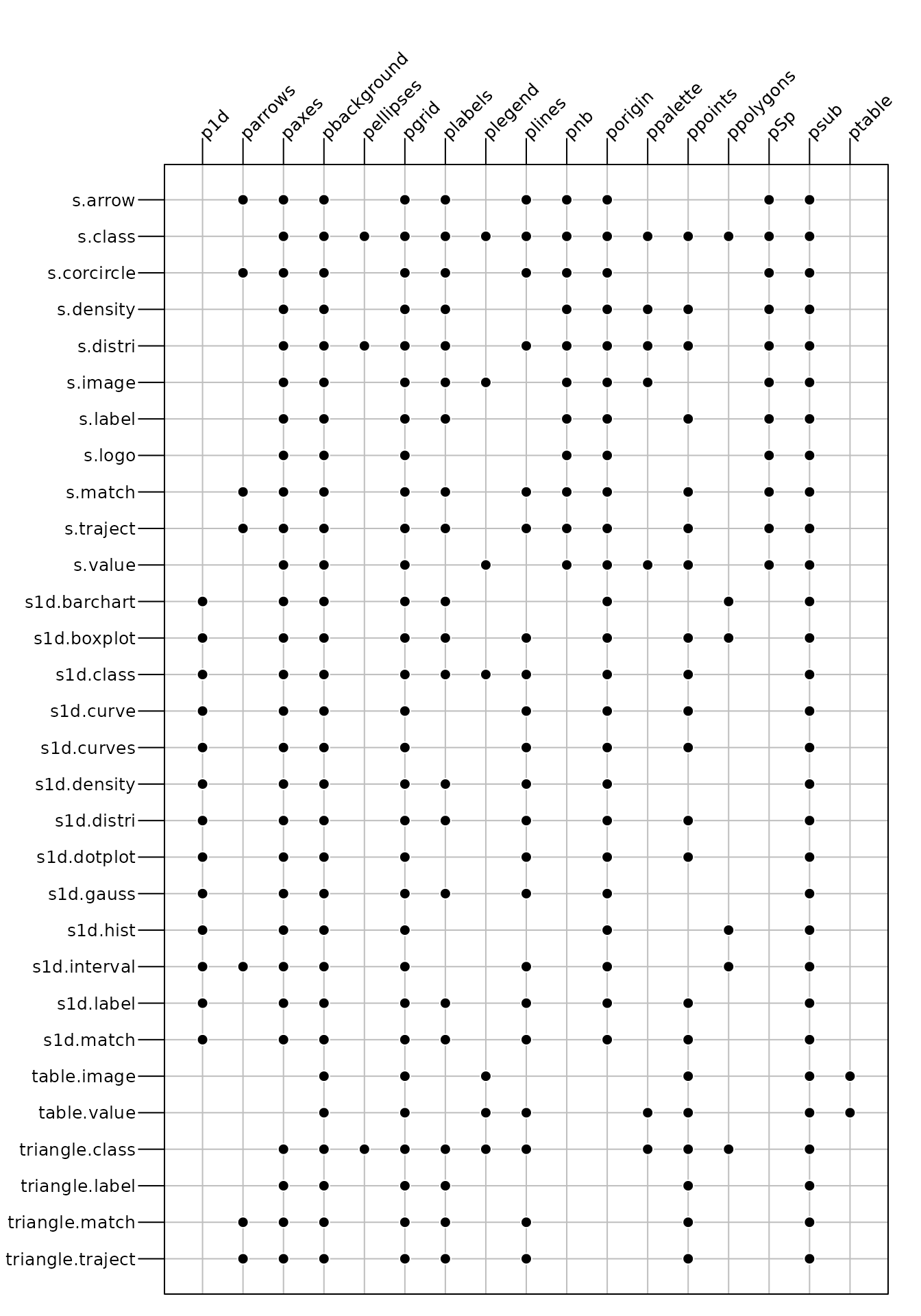
According to the function called, only some of the full list of adeg.par parameters are useful to modify the graphical display. Figure 4 indicates which parameters can affect the display of an object created by a given user function. For example, the background (pbackground parameter) can be modified for all functions whereas the display of ellipses (pellipses parameter) affects only three functions.

Figure 4: Effect of adeg.par parameters in adegraphics functions.

Global assignment

The adegpar function allows to modify globally the values of graphical parameters so that changes will affect all subsequent displays. For example, we update the size/color of labels and add axes to a plot:

oldadegpar <- adegpar()
adegpar("plabels")

## $plabels
## $plabels$alpha
## [1] 1
## 
## $plabels$cex
## [1] 1
## 
## $plabels$col
## [1] "black"
## 
## $plabels$srt
## [1] "horizontal"
## 
## $plabels$optim
## [1] FALSE
## 
## $plabels$boxes
## $plabels$boxes$alpha
## [1] 1
## 
## $plabels$boxes$border
## [1] "black"
## 
## $plabels$boxes$col
## [1] "white"
## 
## $plabels$boxes$draw
## [1] TRUE
## 
## $plabels$boxes$lwd
## [1] 1
## 
## $plabels$boxes$lty
## [1] 1

g13 <- s.label(dfxy = pca1$li, plot = FALSE)
adegpar(plabels = list(col = "blue", cex = 1.5), paxes.draw = TRUE)
adegpar("plabels")

## $plabels
## $plabels$alpha
## [1] 1
## 
## $plabels$cex
## [1] 1.5
## 
## $plabels$col
## [1] "blue"
## 
## $plabels$srt
## [1] "horizontal"
## 
## $plabels$optim
## [1] FALSE
## 
## $plabels$boxes
## $plabels$boxes$alpha
## [1] 1
## 
## $plabels$boxes$border
## [1] "black"
## 
## $plabels$boxes$col
## [1] "white"
## 
## $plabels$boxes$draw
## [1] TRUE
## 
## $plabels$boxes$lwd
## [1] 1
## 
## $plabels$boxes$lty
## [1] 1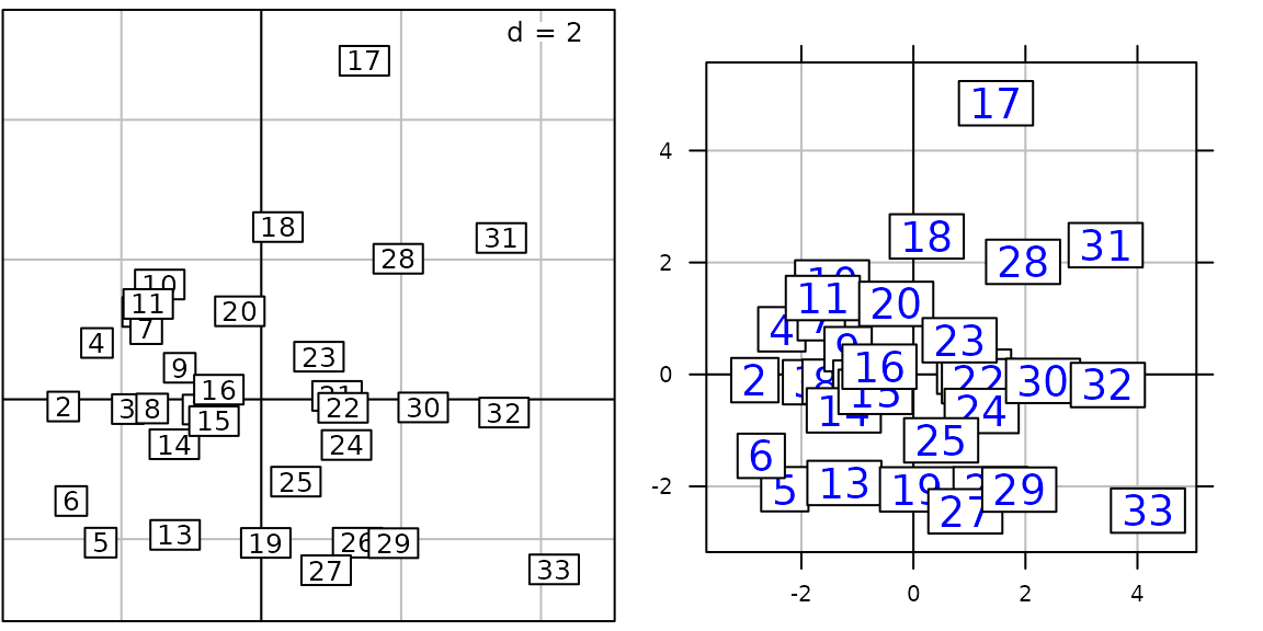

g14 <- s.label(dfxy = pca1$li, plot = FALSE)
ADEgS(c(g13, g14), layout = c(1, 2))

As the adegpar function can accept numerous graphical parameters, it can be used to define some graphical themes. The next releases of adegraphics will offer functionalities to easily create, edit and store graphical themes. Here, we reassign the original default parameters:

adegpar(oldadegpar)

Local assignment

A second option is to update the graphical parameters locally so that the changes will only modify the object created. This is done using the dots (...) argument in the call to a user function. In this case, the default values of parameters in the global environment are not modified:

adegpar("ppoints")

## $ppoints
## $ppoints$alpha
## [1] 1
## 
## $ppoints$cex
## [1] 1
## 
## $ppoints$col
## [1] "black"
## 
## $ppoints$pch
## [1] 20
## 
## $ppoints$fill
## [1] "black"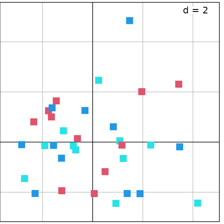

s.label(dfxy = pca1$li, plabels.cex = 0, ppoints = list(col = c(2, 4, 5), cex = 1.5, pch = 15))

adegpar("ppoints")

## $ppoints
## $ppoints$alpha
## [1] 1
## 
## $ppoints$cex
## [1] 1
## 
## $ppoints$col
## [1] "black"
## 
## $ppoints$pch
## [1] 20
## 
## $ppoints$fill
## [1] "black"

In the previous example, we can see that parameters can be either specified using a ’.’ separator or a list. For instance, using plabels.cex = 0 or plabels = list(cex = 0) is strictly equivalent. Moreover, partial names can be used if there is no ambiguity (such as plab.ce = 0 in our example).

Parameters in `g.args`

The g.args slot is a list of parameters specific to the function used (and thus to the class of the returned object). Several parameters are very general and used in all adegraphics functions:

xlim, ylim: limits of the graph on the x and y axes
main, sub: main title and subtitle
xlab, ylab: labels of the x and y axes
scales: a list determining how the x and y axes (tick marks dans labels) are drawn; this is the scales parameter of the xyplot function of lattice

The ADEg.S2 objects can also contain spatial information (map stored as a Spatial object or neighborhood stored as a nb object):

Sp, sp.layout: objects from the sp package to display spatial objects, Sp for maps and sp.layout for spatial widgets as a North arrow, scale, etc.
nbobject: object of class nb or listw to display neighbor graphs.

When the facets (see the Partitioning the data (facets) section) argument is used, users can modify the parameter samelimits: if it is TRUE, all graphs have the same limits whereas limits are computed for each subgraph independently when it is FALSE. For example, considering the jv73 data set, each subgraph is computed with its own limits and labels are then more scattered:

s.label(pca2$li, facets = jv73$fac.riv, samelimits = FALSE)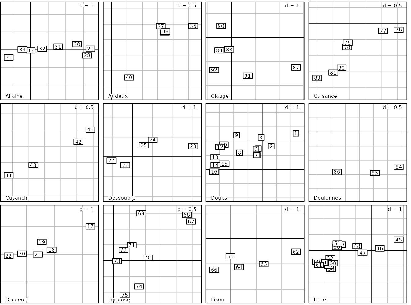

Several other g.args parameters can be updated according to the class of the created object (see Figure 2).

Parameters applied on a `ADEgS`

Users can either apply the changes to all graphs or to update only one graph. Of an ADEgS, to apply changes on all the graphs contained in an ADEgS, the syntax is similar to the one described for an ADEg object. For example, background color can be changed for all graphs in g10 using the pbackground.col parameter.

g15 <- plot(coi1, pbackground.col = "steelblue")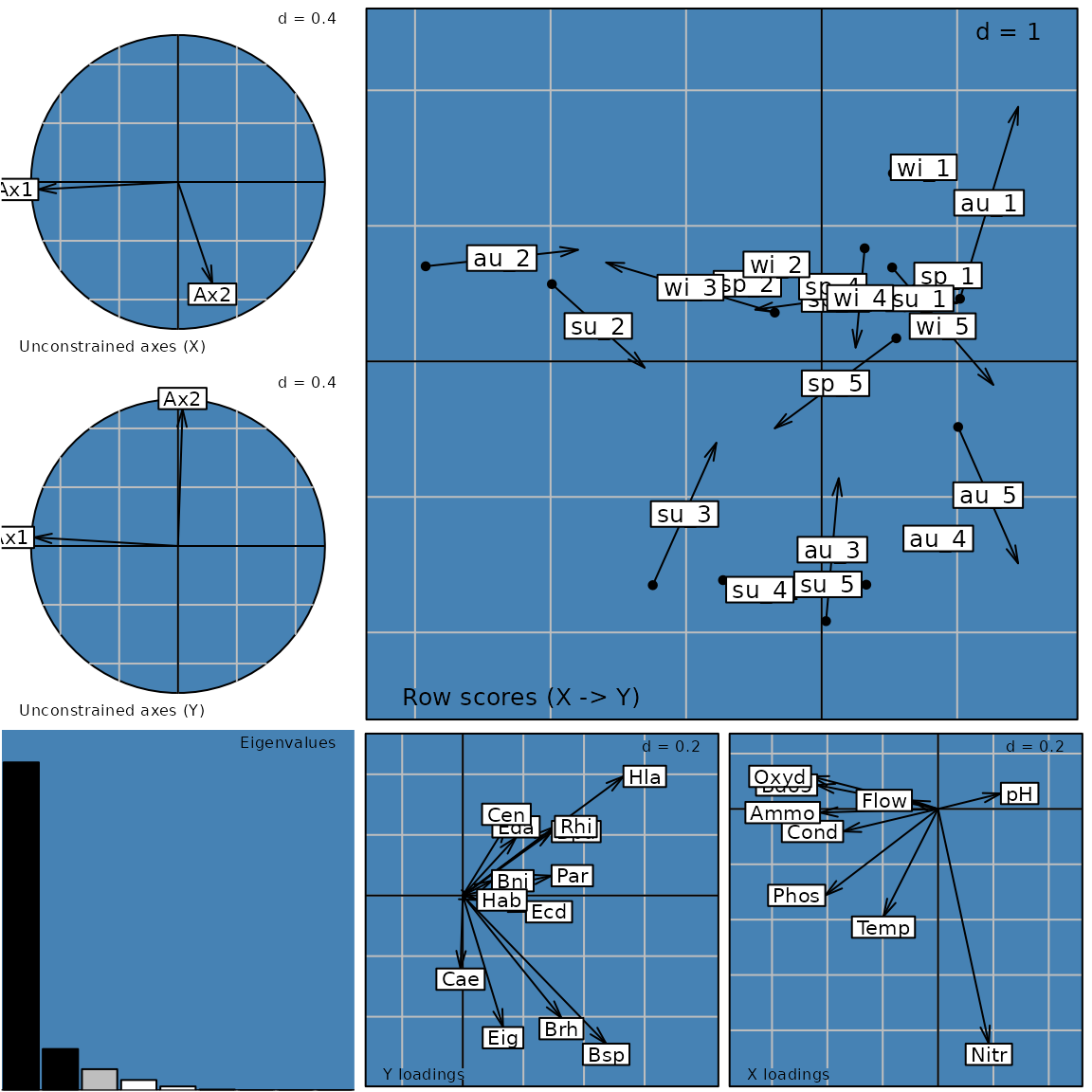

To change the parameters of a given graph, the name of the parameter must be preceded by the name of the subgraph. This supposes that the names of subgraphs are known. For example, to modify only two graphs:

names(g15)

## [1] "Xax"       "Yax"       "eig"       "XYmatch"   "Yloadings" "Xloadings"

plot(coi1, XYmatch.pbackground.col = "steelblue",  XYmatch.pgrid.col = "red", 
     eig.ppolygons.col = "orange")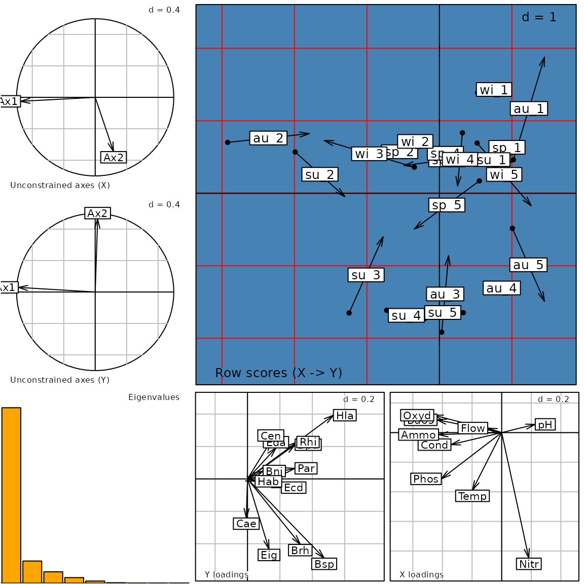

Using `adegraphics` functions in your package

In this section, we illustrate how adegraphics functionalities can be used to implement graphical functions in your own package. We created an objet of class track that contains a vector of distance and time.

tra1 <- list()
tra1$time <- runif(300)
tra1$distance <- tra1$time * 5 + rnorm(300)
class(tra1) <- "track"

For an object of the class track, we wish to represent different components of the data:

an histogram of distances
an histogram of speeds (i.e., distance / time)
a 2D plot representing the distance, the time and the line corresponding to the linear model that predict distance by time

The corresponding multiple plot can be done using adegraphics functions:

g1 <- s1d.hist(tra1$distance, psub.text = "distance", ppolygons.col = "blue", 
               pgrid.draw = FALSE, plot = FALSE)
g2 <- s1d.hist(tra1$distance / tra1$time, psub.text = "speed", ppolygons.col = "red", 
               plot = FALSE)
g31 <- s.label(cbind(tra1$time, tra1$distance), paxes = list(aspectratio = "fill", 
               draw = TRUE), plot = FALSE)
g32 <- xyplot(tra1$distance ~ tra1$time, aspect = g31@adeg.par$paxes$aspectratio, 
              panel = function(x, y) {panel.lmline(x, y)})
g3 <- superpose(g31, g32)
G <- ADEgS(list(g1, g2, g3))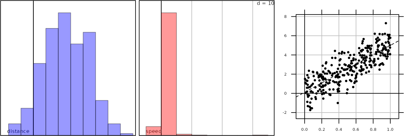

To facilitate the graphical representation of an object of class track, the simplest solution is to design a function plot for this class. We illustrate how to define such function with a particular emphasis on the management of graphical parameters. The function is provided below and we detail the different steps.

plot.track <- function(x, pos = -1, storeData = TRUE, plot = TRUE, ...) {
 
 ## step 1 : sort parameters for each graph
 graphsnames <- c("histDist", "histSpeed", "regression")
 sortparameters <- sortparamADEgS(..., graphsnames = graphsnames, 
                                  nbsubgraphs = c(1, 1, 2))
 
 ## step 2 : define default values for graphical parameters
 params <- list()
 params[[1]] <- list(psub = list(text = "distance"), ppolygons = list(col = "blue"), 
                     pgrid = list(draw = FALSE))
 params[[2]] <- list(psub = list(text = "speed"), ppolygons = list(col = "red"), 
                     pgrid = list(draw = FALSE))
 params[[3]] <- list()
 params[[3]]$l1 <- list(paxes = list(aspectratio = "fill", draw = TRUE))
 params[[3]]$l2 <- list()
 names(params) <- graphsnames
 sortparameters <- modifyList(params, sortparameters, keep.null = TRUE)
 
 ## step 3 : create each individual plot (ADEg)
 g1 <- do.call("s1d.hist", c(list(score = substitute(x$distance), plot = FALSE, 
               storeData = storeData, pos = pos - 2), sortparameters[[1]]))
 g2 <- do.call("s1d.hist", c(list(score = substitute(x$distance / x$time), 
               plot = FALSE, storeData = storeData, pos = pos - 2), sortparameters[[2]]))
 g31 <- do.call("s.label", c(list(dfxy = substitute(cbind(x$time, x$distance)), plot = 
               FALSE, storeData = storeData, pos = pos - 2), sortparameters[[3]][[1]]))
 g32 <- xyplot(x$distance ~ x$time, aspect = g31@adeg.par$paxes$aspectratio,
               panel = function(x, y) {panel.lmline(x, y)})
 g3 <- do.call("superpose", list(g31, g32))
 g3@Call <- call("superpose", g31@Call, g32$call)
 
 
 ## step 4 : create the multiple plot (ADEgS)
 lay <- matrix(1:3, 1, 3)
 object <- new(Class = "ADEgS", ADEglist = list(g1, g2, g3), positions = 
               layout2position(lay), add = matrix(0, ncol = 3, nrow = 3), 
               Call = match.call())
 names(object) <- graphsnames
 if(plot)
   print(object)
 invisible(object)
}

In the first step, the arguments given by the user through the dots (…) argument are managed. A name is given to each subgraph and stored in the vector graphnames. Then, the function sortparamADEgS associates the graphical parameters of the dots (…) argument to each subgraph. If a prefix is specified and matches the name of a graph (e.g., histDist.pbackground.col = grey), the parameter is applied only to the graphic specified (e.g., called histDist). If no prefix is specified (e.g., pbackground.col = grey), the parameter is applied to all subgraphs. The function sortparamADEgS returns a list (length equal to the number of subgraph) of lists of graphical parameters.

In the second step, default values for some graphical parameters are modified. The default parameters are stored in a list which has the same structure that the one produced by sortparamADEgS (i.e., names corresponding to those contained in graphsnames). Then, the modifyList function is applied to merge user and defaults values of paramaters (if a parameter is specified by the user and in the default, the value given by the user is used).

In the third step, each subgraph is created. Here, we create two C1.hist objects and superpose a S2.label object and a trellis one. The functions do.call and substitute are used to provide a pretty call for each subgraph (stored in the Call slot).

In a final step, the multiple graph is build through the creation of a new ADEgS object and possibly plotted.

The plot.track function can then be used by:

plot(tra1)

Graphical parameters can be modified by:

plot(tra1, histDist.ppoly.col = "green", pbackground.col = "grey")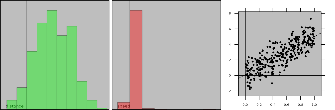

Examples

Labels customization

data(meaudret)
g16 <- s.label(pca3$li, plot = FALSE)
g17 <- s.label(pca3$li, ppoints.col= "red", plabels = list(box = list(draw = FALSE), 
  optim = TRUE), plot = FALSE)
ADEgS(c(g16, g17), layout = c(1, 2))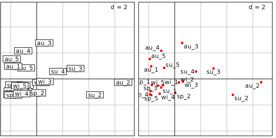

Ellipses, stars and convex hulls

g18 <- s.class(pca3$li, fac = meaudret$design$season, plot = FALSE)
g19 <- s.class(pca3$li, fac = meaudret$design$season, ellipseSize = 0, 
  chullSize = 1, starSize = 0.5, col = TRUE, plot = FALSE)
g20 <- s.class(pca3$li, fac = meaudret$design$season, pellipses.lwd = 2, 
  pellipses.border = 2:5, pellipses.col = 2:5, plot = FALSE)
g21 <- s.class(pca3$li, fac = meaudret$design$season, ellipseSize = 0, 
  chullSize = 0, ppolygons.lwd = 2, plines.col = 2:5, starSize = 1.2, plot = FALSE)
ADEgS(c(g18, g19, g20, g21), layout = c(2, 2))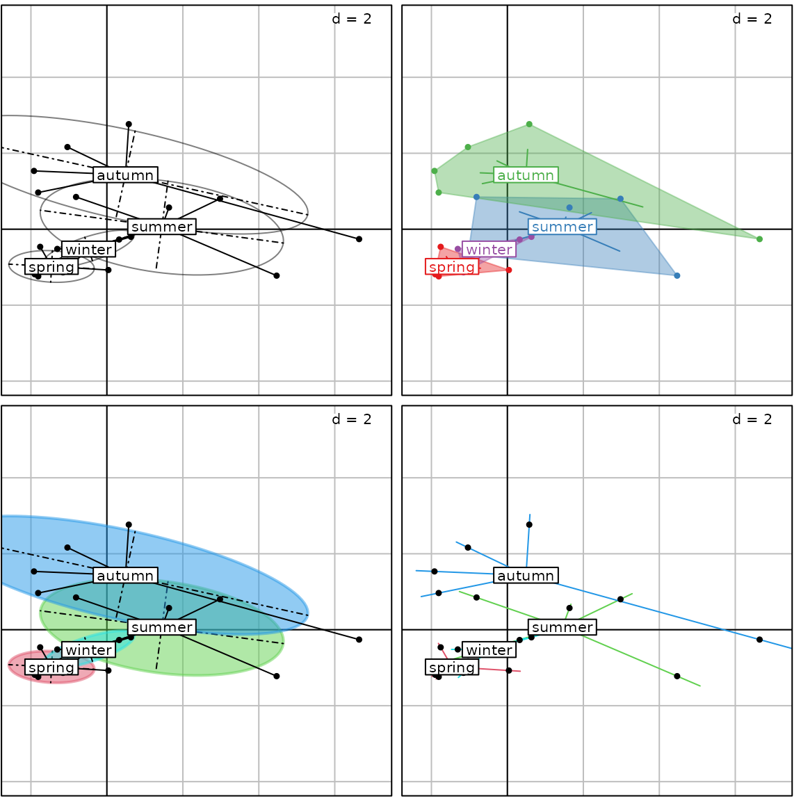

Values and legend

data(rpjdl)
coa2 <- dudi.coa(rpjdl$fau, scannf = FALSE, nf = 3)
g22 <- s.value(coa2$li, coa2$li[,3], plot = FALSE)
g23 <- s.value(coa2$li, coa2$li[,3], method = "color", ppoints.cex = 0.8, 
  plegend.size= 0.8, plot = FALSE)
g24 <- s.value(coa2$li, coa2$li[,3], plegend.size = 0.8, ppoints.cex = 0.8, 
  symbol = "square", method = "color", key = list(columns = 1), 
  col = colorRampPalette(c("yellow", "blue"))(6), plot = FALSE)
g25 <- s.value(coa2$li, coa2$li[, 3], center = 0, method = "size", ppoints.cex = 0.6, 
  symbol = "circle", col = c("yellow", "red"), plot = FALSE)
ADEgS(c(g22, g23, g24, g25), layout = c(2, 2))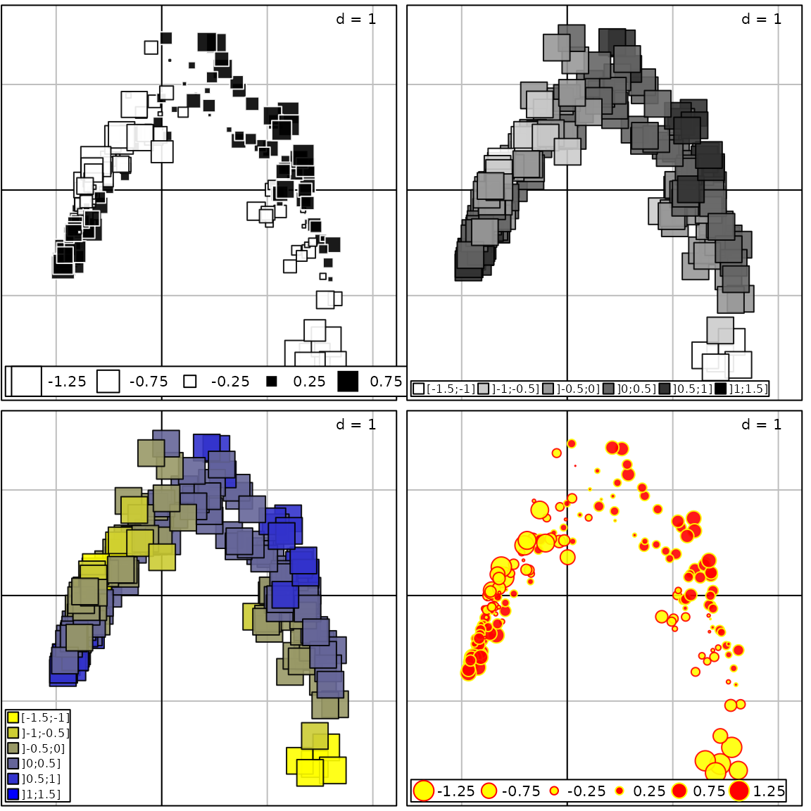

1-D plot

score1 <- c(rnorm(1000, mean = -0.5, sd = 0.5), rnorm(1000, mean = 1))
fac1 <- rep(c("A", "B"), each = 1000)
g26 <- s1d.density(score1, fac1, pback.col = "grey75", plot = FALSE)
g27 <- s1d.density(score1, fac1, col = c(2, 4), plot = FALSE)
g28 <- s1d.density(score1, fac1, col = c(2, 4), p1d.reverse = TRUE, p1d.horizontal = FALSE, 
  p1d.rug.draw = FALSE, plot = FALSE)
g29 <- s1d.density(score1, fac1, col = c(2, 4), ppolygons.alpha = 0.2, 
  p1d = list(rug = list(tck = 1, line = FALSE)), plot = FALSE)
ADEgS(c(g26, g27, g28, g29), layout = c(2, 2))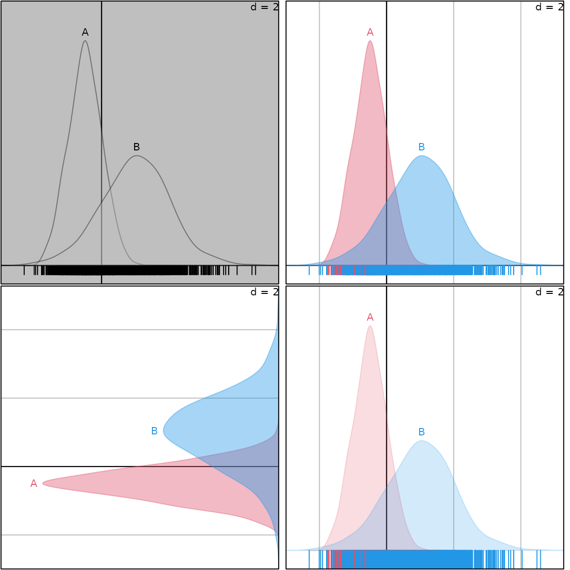

Maps and neighbor graphs

if(require(Guerry)) {
  library(sp)
  data(gfrance85)
  region.names <- data.frame(gfrance85)[, 5]
  col.region <- colors()[c(149, 254, 468, 552, 26)]
  g30 <- s.class(coordinates(gfrance85), region.names, porigin.include = FALSE, plot = FALSE)
  g31 <- s.class(coordinates(gfrance85), region.names, ellipseSize = 0, starSize = 0,
                 Sp = gfrance85, pgrid.draw = FALSE, pSp.col = col.region[region.names], pSp.alpha = 0.4,
                 plot = FALSE)
  ADEgS(c(g30, g31), layout = c(1, 2))
}

## Loading required package: Guerry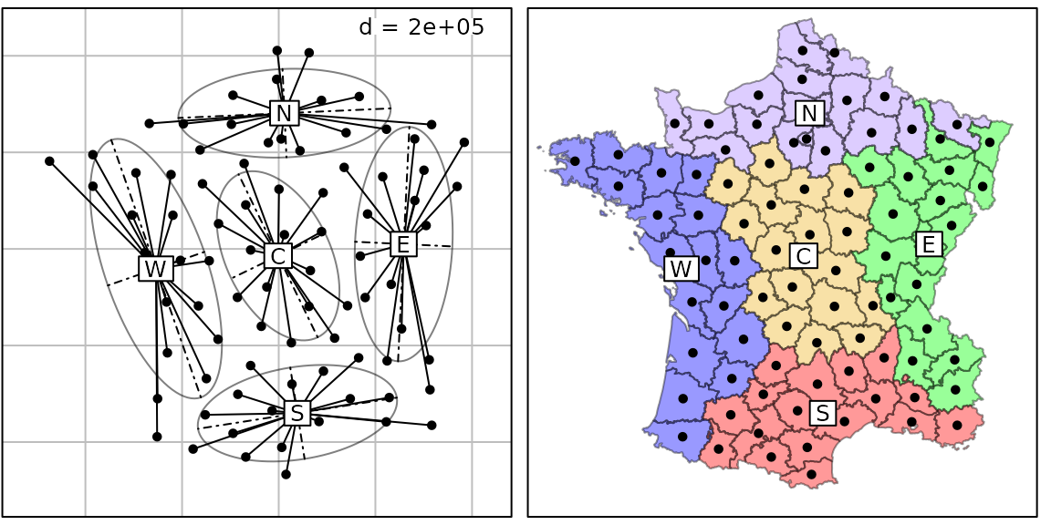

# if(require(Guerry)) {
#   s.Spatial(gfrance85[,7:12])
# }

data(mafragh, package = "ade4")
g32 <- s.label(mafragh$xy, nb = mafragh$nb, plot = FALSE)
g33 <- s.label(mafragh$xy, nb = mafragh$nb, pnb.ed.col = "red", plab.cex = 0, 
  pnb.node = list(cex = 3, col = "blue"), ppoints.col = "green", plot = FALSE)
ADEgS(c(g32, g33), layout = c(1, 2))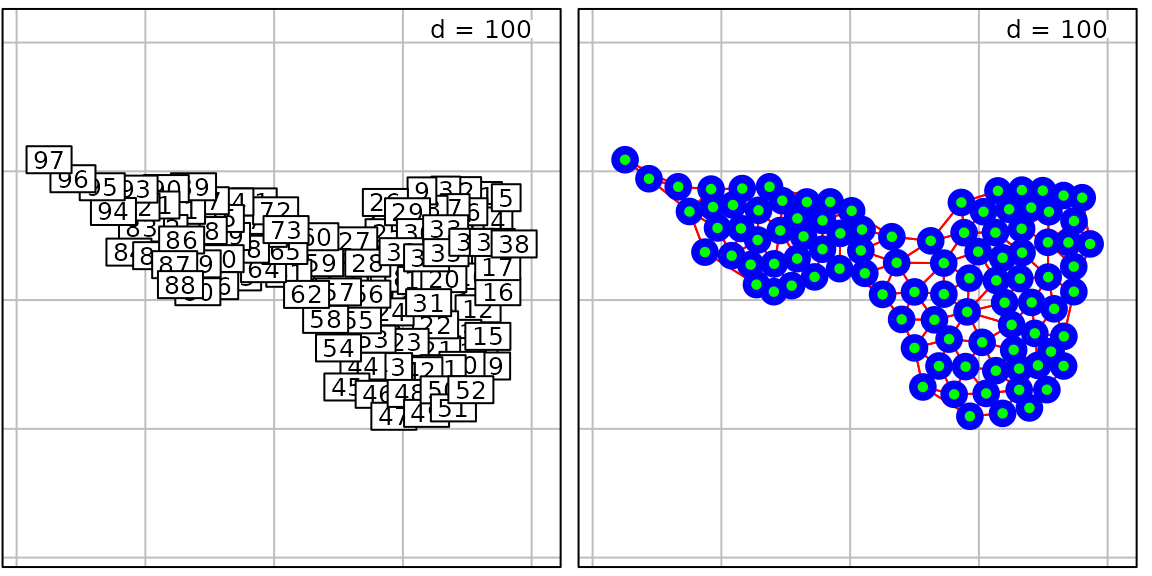

Ternary plots

data(euro123, package = "ade4")
df <- rbind.data.frame(euro123$in78, euro123$in86, euro123$in97)
row.names(df) <- paste(row.names(euro123$in78), rep(c(1, 2, 3), rep(12, 3)), sep = "")
g34 <- triangle.label(df, label = row.names(df), showposition = TRUE, plot = FALSE)
g35 <- triangle.label(euro123$in78, plabels.cex = 0, ppoints.cex = 2, addmean = TRUE, 
  show = FALSE, plot = FALSE)
ADEgS(c(g34, g35), layout = c(1, 2))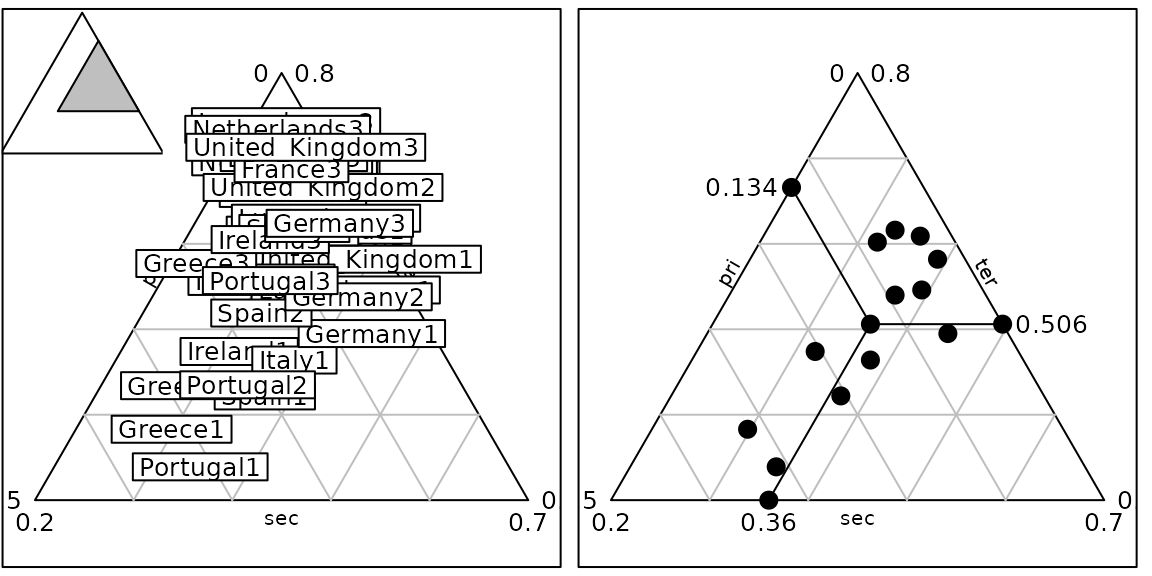

Appendix

This appendix summarizes the main changes between ade4 and adegraphics. Each line corresponds to a graphical argument defined in ade4 and its equivalent in adegraphics is given.

Arguments in `ade4`	Functions in `ade4`	`g.args` in `adegraphics`	`adeg.par` in `adegraphics`
`abline.x`	`table.cont`	`ablineX`
`abline.y`	`table.cont`	`ablineY`
`abmean.x`	`table.cont`	`meanX`
`abmean.y`	`table.cont`	`meanY`
`addaxes`	`s.arrow`, `s.chull`, `s.class`, `s.distri`, `s.image`, `s.kde2d`, `s.label`, `s.logo`, `s.match`, `s.traject`, `s.value`, `triangle.class`, `triangle.plot`		`paxes.draw`
`area`	`s.arrow`, `s.chull`, `s.class`, `s.distri`, `s.image`, `s.kde2d`, `s.label`, `s.logo`, `s.match`, `s.traject`, `s.value`	`Sp`		a `Sp` object
`axesell`	`s.class`, `s.distri`, `triangle.class`		`pellipses.axes.draw`
`box`	`s.corcircle`, `triangle.plot`		`pbackground.box`
`boxes`	`s.arrow`, `s.label`, `sco.class`, `sco.label`, `sco.match`		`plabels.boxes.draw`
`cellipse`	`s.class`, `s.distri`, `triangle.class`	`ellipseSize`
`cgrid`	`s.arrow`, `s.class`, `s.chull`, `s.corcircle`, `s.distri`, `s.image`, `s.kde2d`, `s.label`, `s.logo`, `s.match`, `s.traject`, `s.value`, `sco.boxplot`, `sco.class`, `sco.distri`, `sco.gauss`, `sco.label`, `sco.match`		`pgrid.nint`	both play on the grid mesh, but they are not strictly equivalent
`clabel`	`s.arrow`, `s.class`, `s.chull`, `s.corcircle`, `s.distri`, `s.kde2d`, `s.label`, `s.match`, `s.traject`, `sco.boxplot`, `sco.class`, `sco.distri`, `sco.gauss`, `sco.label`, `sco.match`, `triangle.plot`		`plabels.cex`
`clabel`	`table.dist`			`axis.text = list()` `lattice` parameter
`clabel.col`	`table.cont`, `table.paint`, `table.value`			`axis.text = list()` `lattice` parameter
`clabel.row`	`table.cont`, `table.paint`, `table.value`			`axis.text = list()` `lattice` parameter
`clegend`	`s.value`, `table.cont`, `table.value`		`plegend.size` `ppoints.cex`	parameters setting the legend size
`clegend`	`table.paint`		`plegend.size`
`clogo`	`s.logo`		`ppoints.cex`
`cneig`	`s.image`, `s.kde2d`, `s.label`, `s.logo`, `s.value`		`pnb.edge.lwd`
`col.labels`	`table.cont`, `table.paint`, `table.value`	`labelsy`
`contour`	`s.arrow`, `s.class`, `s.chull`, `s.distri`, `s.image`, `s.kde2d`, `s.label`, `s.logo`, `s.match`, `s.traject`, `s.value`	`Sp`		a `Sp` object
`contour.plot`	`s.image`	`region`
`cpoints`, `cpoint`	`s.arrow`, `s.class`, `s.chull`, `s.distri`, `s.kde2d`, `s.label`, `s.match`, `s.traject`, `s.value`, `sco.class`, `sco.label`, `sco.match`, `triangle.class`, `triangle.plot`		`ppoints.cex`
`csize`	`s.value`, `table.cont`, `table.dist`, `table.paint`, `table.value`	`ppoints.cex`
`csize`	`sco.distri`	`sdSize`
`cstar`	`s.class`, `s.distri`, `triangle.class`	`starSize`
`csub`	`s.arrow`, `s.chull`, `s.class`, `s.corcircle`, `s.distri`, `s.image`, `s.kde2d`, `s.label`, `s.logo`, `s.match`, `s.traject`, `s.value`, `sco.boxplot`, `sco.class`, `sco.distri`, `sco.gauss`, `sco.label`, `sco.match`, `triangle.class`, `triangle.plot`		`psub.cex`
`draw.line`	`triangle.biplot`, `triangle.class`, `triangle.plot`		`pgrid.draw`
`edge`	`s.arrow`, `s.match`, `s.traject`		`parrows.length`	setting the length of the arrows to 0 is equivalent to `edge = FALSE`
`grid`	`s.arrow`, `s.chull`, `s.class`, `s.corcircle`, `s.distri`, `s.image`, `s.kde2d`, `s.label`, `s.logo`, `s.match`, `s.traject`, `s.value`, `sco.boxplot`, `sco.class`, `sco.distri`, `sco.gauss`, `sco.label`, `sco.match`, `table.cont`, `table.dist`, `table.value`		`pgrid.draw`
`horizontal`	`sco.class`, `sco.gauss`, `sco.label`, `sco.match`		`p1d.horizontal`
`image.plot`	`s.image`	`contour`
`includeorigin`, `include.origin`	`s.arrow`, `s.chull`, `s.class`, `s.distri`, `s.image`, `s.kde2d`, `s.label`, `s.logo`, `s.match`, `s.traject`, `s.value`, `sco.boxplot`, `sco.class`, `sco.distri`, `sco.gauss`, `sco.label`, `sco.match`		`porigin.include`
`kgrid`	`s.image`	`gridsize`
`klogo`	`s.logo`			no correspondence
`labeltriangle`	`triangle.class` , `triangle.plot`			no correspondence
`legen`	`sco.gauss`	`labelplot`
`neig`	`s.image`, `s.kde2d`, `s.label`, `s.logo`, `s.value`	`nbobject`		a `nb` object
`optchull`	`s.chull`	`chullSize`
`origin`	`s.arrow`, `s.chull`, `s.class`, `s.corcircle`, `s.distri`, `s.image`, `s.kde2d`, `s.label`, `s.logo`, `s.match`, `s.traject`, `s.value`, `sco.boxplot`, `sco.class`, `sco.distri`, `sco.gauss`, `sco.label`, `sco.match`		`porigin.origin`
`pch`	`s.arrow`, `s.chull`, `s.class`, `s.distri`, `s.kde2d`, `s.label`, `s.match`, `s.traject`, `s.value`, `sco.boxplot`, `sco.class`, `sco.label`, `sco.match`, `triangle.class`, `triangle.plot`, `table.cont`		`ppoints.pch`
`pixmap`	`s.arrow`, `s.chull`, `s.class`, `s.distri`, `s.image`, `s.kde2d`, `s.label`, `s.logo`, `s.match`, `s.traject`, `s.value`			no correspondence
`pos.lab`	`sco.class`, `sco.label`, `sco.match`		`p1d.labpos`
`possub`	`s.arrow`, `s.chull`, `s.class`, `s.corcircle`, `s.distri`, `s.image`, `s.kde2d`, `s.label`, `s.logo`, `s.match`, `s.traject`, `s.value`, `sco.class`, `sco.gauss`, `sco.label`, `sco.match`, `triangle.class`, `triangle.plot`		`psub.pos`
`rectlogo`	`s.logo`	`rect`
`reverse`	`sco.class`, `sco.gauss`, `sco.label`, `sco.match`		`p1d.reverse`
`row.labels`	`table.cont`, `table.paint`, `table.value`	`labelsx`
`scale`	`triangle.class`, `triangle.plot`	`adjust`
`show.position`	`triangle.class`, `triangle.plot`	`showposition`
`sub`	`s.arrow`, `s.chull`, `s.class`, `s.corcircle`, `s.distri`, `s.image`, `s.kde2d`, `s.label`, `s.logo`, `s.match`, `s.traject`, `s.value`, `sco.boxplot`, `sco.class`, `sco.distri`, `sco.gauss`, `sco.label`, `sco.match`, `triangle.class`, `triangle.plot`		`psub.text`
`y.rank`	`sco.distri`	`yrank`
`zmax`	`s.value`			set to default max(abs(z))

References

Dray, Stéphane, and Anne-Béatrice Dufour. 2007. “The ade4 Package: Implementing the Duality Diagram for Ecologists.” Journal of Statistical Software 22 (4): 1–20. https://doi.org/10.18637/jss.v022.i04.

Murrell, Paul. 2005. R Graphics. Chapman & Hall/CRC Press. https://www.e-reading.club/bookreader.php/137370/C486x_APPb.pdf.

Sarkar, Deepayan. 2008. Lattice: Multivariate Data Visualization with r. Springer. https://doi.org/10.1007/978-0-387-75969-2.

Siberchicot, Aurélie, Alice Julien-Laferrière, Anne-Béatrice Dufour, Jean Thioulouse, and Stéphane Dray. 2017. “adegraphics: An S4 Lattice-Based Package for the Representation of Multivariate Data.” The R Journal 9 (2): 198–212. https://journal.r-project.org/archive/2017/RJ-2017-042/index.html.

Alice Julien-Laferrière, Aurélie Siberchicot and Stéphane Dray

2025-04-07

An overview of object classes

Simple graph (`ADEg` object)

User functions

Arguments

Slots and Methods

Multiple graph (`ADEgS` object)

Slots and Methods

Creating an `ADEgS` object by hand

The basic methods for superposition, juxtaposition and insertion

The `ADEgS` function

Automatic collections

Partitioning the data (`facets`)

Multiple axes

Multiple score

Multiple variable

Outputs of the `ade4` package

Customizing a graph

Parameters in `trellis.par`

Parameters in `adeg.par`

Global assignment

Local assignment

Parameters in `g.args`

Parameters applied on a `ADEgS`

Using `adegraphics` functions in your package

Examples

Labels customization

Ellipses, stars and convex hulls

Values and legend

1-D plot

Maps and neighbor graphs

Ternary plots

Appendix

References

The `adegraphics` package

Alice Julien-Laferrière, Aurélie Siberchicot and Stéphane Dray

2025-04-07

An overview of object classes

Simple graph (ADEg object)

User functions

Arguments

Slots and Methods

Multiple graph (ADEgS object)

Slots and Methods

Creating an ADEgS object by hand

The basic methods for superposition, juxtaposition and insertion

The ADEgS function

Automatic collections

Partitioning the data (facets)

Multiple axes

Multiple score

Multiple variable

Outputs of the ade4 package

Customizing a graph

Parameters in trellis.par

Parameters in adeg.par

Global assignment

Local assignment

Parameters in g.args

Parameters applied on a ADEgS

Using adegraphics functions in your package

Examples

Labels customization

Ellipses, stars and convex hulls

Values and legend

1-D plot

Maps and neighbor graphs

Ternary plots

Appendix

References

Simple graph (`ADEg` object)

Multiple graph (`ADEgS` object)

Creating an `ADEgS` object by hand

The `ADEgS` function

Partitioning the data (`facets`)

Outputs of the `ade4` package

Parameters in `trellis.par`

Parameters in `adeg.par`

Parameters in `g.args`

Parameters applied on a `ADEgS`

Using `adegraphics` functions in your package