Class of the Permutation Tests (in C).

randtest is a generic function. It proposes methods for the following objects between, discrimin, coinertia ...

Usage

randtest(xtest, ...)
as.randtest(sim, obs, alter = c("greater", "less", "two-sided"), 
  output = c("light", "full"), call = match.call(), subclass = NULL)

# S3 method for class 'randtest'
plot(x, nclass = 10, coeff = 1, ...)
# S3 method for class 'randtest'
print(x, ...)

Arguments

xtest: an object used to select a method
x: an object of class randtest
...: further arguments passed to or from other methods; in plot.randtest to hist
output: a character string specifying if all simulations should be stored ("full"). This was the default until ade4 1.7-5. Now, by default ("light"), only the distribution of simulated values is stored in element plot as produced by the hist function.
nclass: a number of intervals for the histogram. Ignored if object output is "light"
coeff: to fit the magnitude of the graph. Ignored if object output is "light"
sim: a numeric vector of simulated values
obs: a numeric vector of an observed value
alter: a character string specifying the alternative hypothesis, must be one of "greater" (default), "less" or "two-sided"
call: a call order
subclass: a character vector indicating the subclasses associated to the returned object

Value

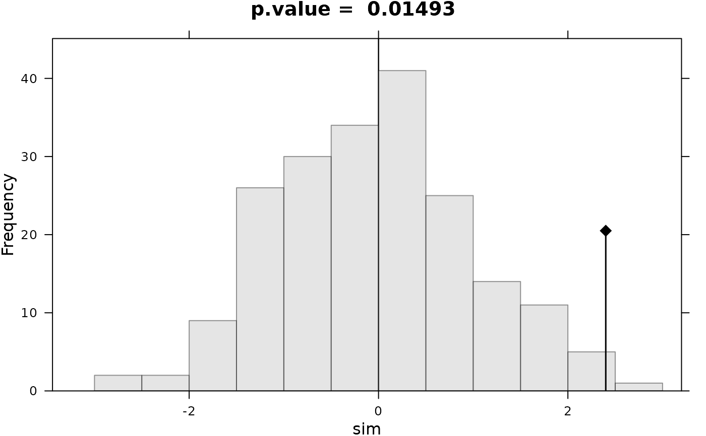
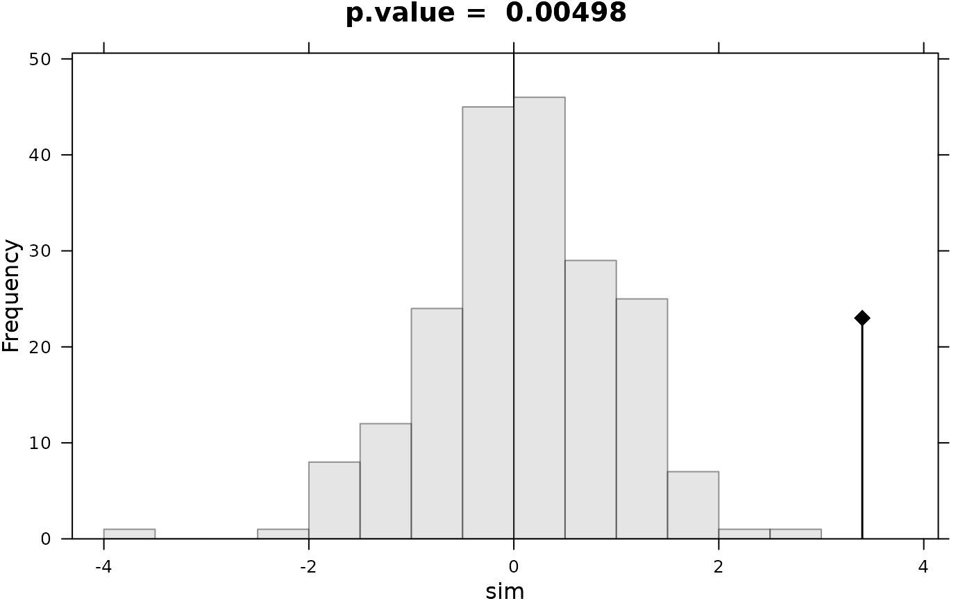
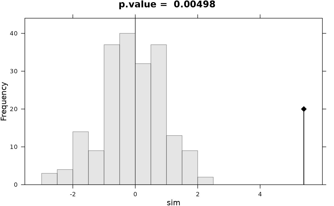
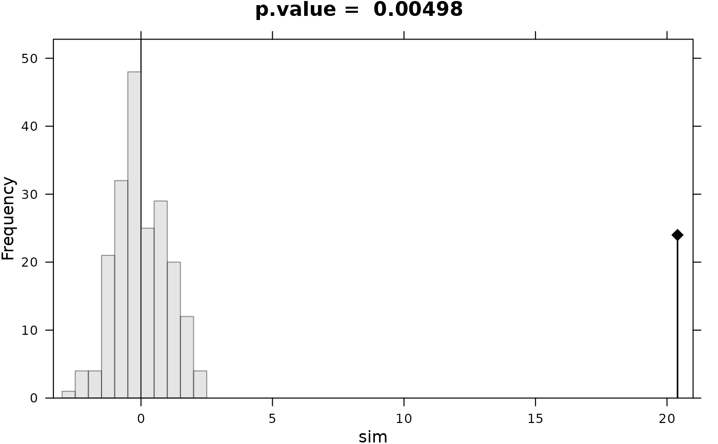
as.randtest returns a list of class randtest.
plot.randtest draws the simulated values histograms and the position of the observed value.

Details

If the alternative hypothesis is "greater", a p-value is estimated as: (number of random values equal to or greater than the observed one + 1)/(number of permutations + 1). The null hypothesis is rejected if the p-value is less than the significance level. If the alternative hypothesis is "less", a p-value is estimated as: (number of random values equal to or less than the observed one + 1)/(number of permutations + 1). Again, the null hypothesis is rejected if the p-value is less than the significance level. Lastly, if the alternative hypothesis is "two-sided", the estimation of the p-value is equivalent to the one used for "greater" except that random and observed values are firstly centered (using the average of random values) and secondly transformed to their absolute values. Note that this is only suitable for symmetric random distribution.

Examples

par(mfrow = c(2,2))
for (x0 in c(2.4,3.4,5.4,20.4)) {
  l0 <- as.randtest(sim = rnorm(200), obs = x0)
  print(l0)
  plot(l0,main=paste("p.value = ", round(l0$pvalue, dig = 5)))
}
#> Monte-Carlo test
#> Call: as.randtest(sim = rnorm(200), obs = x0)
#> 
#> Observation: 2.4 
#> 
#> Based on 200 replicates
#> Simulated p-value: 0.01492537 
#> Alternative hypothesis: greater 
#> 
#>     Std.Obs Expectation    Variance 
#>  2.30501257 -0.03836948  1.11905757 

#> Monte-Carlo test
#> Call: as.randtest(sim = rnorm(200), obs = x0)
#> 
#> Observation: 3.4 
#> 
#> Based on 200 replicates
#> Simulated p-value: 0.004975124 
#> Alternative hypothesis: greater 
#> 
#>     Std.Obs Expectation    Variance 
#>  3.67452167  0.08786151  0.81248500 

#> Monte-Carlo test
#> Call: as.randtest(sim = rnorm(200), obs = x0)
#> 
#> Observation: 5.4 
#> 
#> Based on 200 replicates
#> Simulated p-value: 0.004975124 
#> Alternative hypothesis: greater 
#> 
#>     Std.Obs Expectation    Variance 
#>   5.5211222  -0.1024532   0.9932487 

#> Monte-Carlo test
#> Call: as.randtest(sim = rnorm(200), obs = x0)
#> 
#> Observation: 20.4 
#> 
#> Based on 200 replicates
#> Simulated p-value: 0.004975124 
#> Alternative hypothesis: greater 
#> 
#>      Std.Obs  Expectation     Variance 
#> 20.312870191  0.008292623  1.007777352 

par(mfrow = c(1,1))