Double principal component analysis with respect to instrumental variables

It includes double redundancy analysis (RDA, if dudi argument is created with dudi.pca) and double canonical correspondence analysis (CCA, if dudi argument is created with dudi.coa) as special cases. The function dvaripart computed associated double (by row and column) variation partitioning.

Usage

dpcaiv(dudi, dfR = NULL, dfQ = NULL, scannf = TRUE, nf = 2)
# S3 method for class 'dpcaiv'
plot(x, xax = 1, yax = 2, ...) 
# S3 method for class 'dpcaiv'
print(x, ...)
# S3 method for class 'dpcaiv'
summary(object, ...) 
# S3 method for class 'dpcaiv'
randtest(xtest, nrepet = 99, ...)
dvaripart(Y, dfR, dfQ, nrepet = 999, scale = FALSE, ...)
# S3 method for class 'dvaripart'
print(x, ...)

Arguments

dudi: a duality diagram, object of class dudi
Y: a duality diagram, object of class dudi or a response data.frame
dfR: a data frame with external variables relative to rows of the dudi object
dfQ: a data frame with external variables relative to columns of the dudi object
scannf: a logical value indicating whether the eigenvalues bar plot should be displayed
nf: if scannf FALSE, an integer indicating the number of kept axes

x, object, xtest: an object of class dpcaiv or dvaripart
xax: the column number for the x-axis
yax: the column number for the y-axis
nrepet: an integer indicating the number of permutations
scale: If Y is not a dudi, a logical indicating if variables should be scaled
...: further arguments passed to or from other methods

Value

returns an object of class dpcaiv, sub-class of class dudi

tab: a data frame with the modified array (predicted table)
cw: a numeric vector with the column weigths (from dudi)
lw: a numeric vector with the row weigths (from dudi)
eig: a vector with the all eigenvalues
rank: an integer indicating the rank of the studied matrix
nf: an integer indicating the number of kept axes
c1: a data frame with the Constrained Principal Axes (CPA)
faQ: a data frame with the loadings for Q to build the CPA as a linear combination
li: a data frame with the constrained (by R) row score (LC score)
lsR: a data frame with the unconstrained row score (WA score)
l1: data frame with the Constrained Principal Components (CPC)
faR: a data frame with the loadings for R to build the CPC as a linear combination
co: a data frame with the constrained (by Q) column score (LC score)
lsQ: a data frame with the unconstrained column score (WA score)
call: the matched call
Y: a data frame with the dependant variables
R: a data frame with the explanatory variables for rows
Q: a data frame with the explanatory variables for columns
asR: a data frame with the Principal axes of dudi$tab on CPA
asQ: a data frame with the Principal components of dudi$tab on CPC
corR: a data frame with the correlations between the CPC and R
corQ: a data frame with the correlations between the CPA and Q

References

Rao, C. R. (1964) The use and interpretation of principal component analysis in applied research. Sankhya, A 26, 329–359.

Obadia, J. (1978) L'analyse en composantes explicatives. Revue de Statistique Appliquee, 24, 5–28.

Lebreton, J. D., Sabatier, R., Banco G. and Bacou A. M. (1991) Principal component and correspondence analyses with respect to instrumental variables : an overview of their role in studies of structure-activity and species- environment relationships. In J. Devillers and W. Karcher, editors. Applied Multivariate Analysis in SAR and Environmental Studies, Kluwer Academic Publishers, 85–114.

Ter Braak, C. J. F. (1986) Canonical correspondence analysis : a new eigenvector technique for multivariate direct gradient analysis. Ecology, 67, 1167–1179.

Ter Braak, C. J. F. (1987) The analysis of vegetation-environment relationships by canonical correspondence analysis. Vegetatio, 69, 69–77.

Chessel, D., Lebreton J. D. and Yoccoz N. (1987) Propriétés de l'analyse canonique des correspondances. Une utilisation en hydrobiologie. Revue de Statistique Appliquée, 35, 55–72.

Author

Stéphane Dray stephane.dray@univ-lyon1.fr
Lisa Nicvert

Examples

# example of a double canonical correspondence analysis
data(aviurba)
coa <- dudi.coa(aviurba$fau, scannf = FALSE)
dcca <- dpcaiv(coa, aviurba$mil, aviurba$trait, scannf = FALSE)
dcca
#> Dcouble canonical correspondence analysis
#> call: dpcaiv(dudi = coa, dfR = aviurba$mil, dfQ = aviurba$trait, scannf = FALSE)
#> class: dcaiv dpcaiv dudi 
#> 
#> $rank (rank)     : 8
#> $nf (axis saved) : 2
#> 
#> eigen values: 0.1969 0.08182 0.02968 0.02217 0.01136 ...
#> 
#>  vector length mode    content                
#>  $eig   8      numeric eigen values           
#>  $lw    51     numeric row weigths (from dudi)
#>  $cw    40     numeric col weigths (from dudi)
#> 
#>  data.frame nrow ncol content                          
#>  $Y         51   40   Dependant variables              
#>  $tab       51   40   modified array (predicted table) 
#>  $dfR       51   11   Explanatory variables for rows   
#>  $dfQ       40   4    Explanatory variables for columns
#> 
#>  data.frame nrow ncol content                                             
#>  $c1        40   2    Constrained Principal Axes (CPA)                    
#>  $faQ       9    2    Loadings for Q to build the CPA (linear combination)
#>  $corQ      8    2    Correlations between the CPA and Q                  
#>  $li        51   2    Constrained (by R) row score (LC score)             
#>  $asR       2    2    Principal axis of dudi$tab on CPA                   
#>  $lsR       51   2    Unconstrained row score (WA score)                  
#> 
#>  data.frame nrow ncol content                                             
#>  $l1        51   2    Constrained Principal Components (CPC)              
#>  $faR       18   2    Loadings for R to build the CPC (linear combination)
#>  $corR      17   2    Correlations between the CPC and R                  
#>  $co        40   2    Constrained (by Q) column score (LC score)          
#>  $asQ       2    2    Principal component of dudi$tab on CPC              
#>  $lsQ       40   2    Unconstrained column score (WA score)               
#> 
summary(dcca)
#> Double canonical correspondence analysis
#> 
#> Class: dcaiv dpcaiv dudi
#> Call: dpcaiv(dudi = coa, dfR = aviurba$mil, dfQ = aviurba$trait, scannf = FALSE)
#> 
#> Total inertia: 0.3615
#> 
#> Eigenvalues:
#>     Ax1     Ax2     Ax3     Ax4     Ax5 
#> 0.19687 0.08182 0.02968 0.02217 0.01136 
#> 
#> Projected inertia (%):
#>     Ax1     Ax2     Ax3     Ax4     Ax5 
#>  54.460  22.634   8.211   6.132   3.142 
#> 
#> Cumulative projected inertia (%):
#>     Ax1   Ax1:2   Ax1:3   Ax1:4   Ax1:5 
#>   54.46   77.09   85.30   91.44   94.58 
#> 
#> (Only 5 dimensions (out of 8) are shown)
#> 
#> Total unconstrained inertia (coa): 2.659
#> 
#> Inertia of coa explained by aviurba$mil and aviurba$trait (%): 13.59
#> 
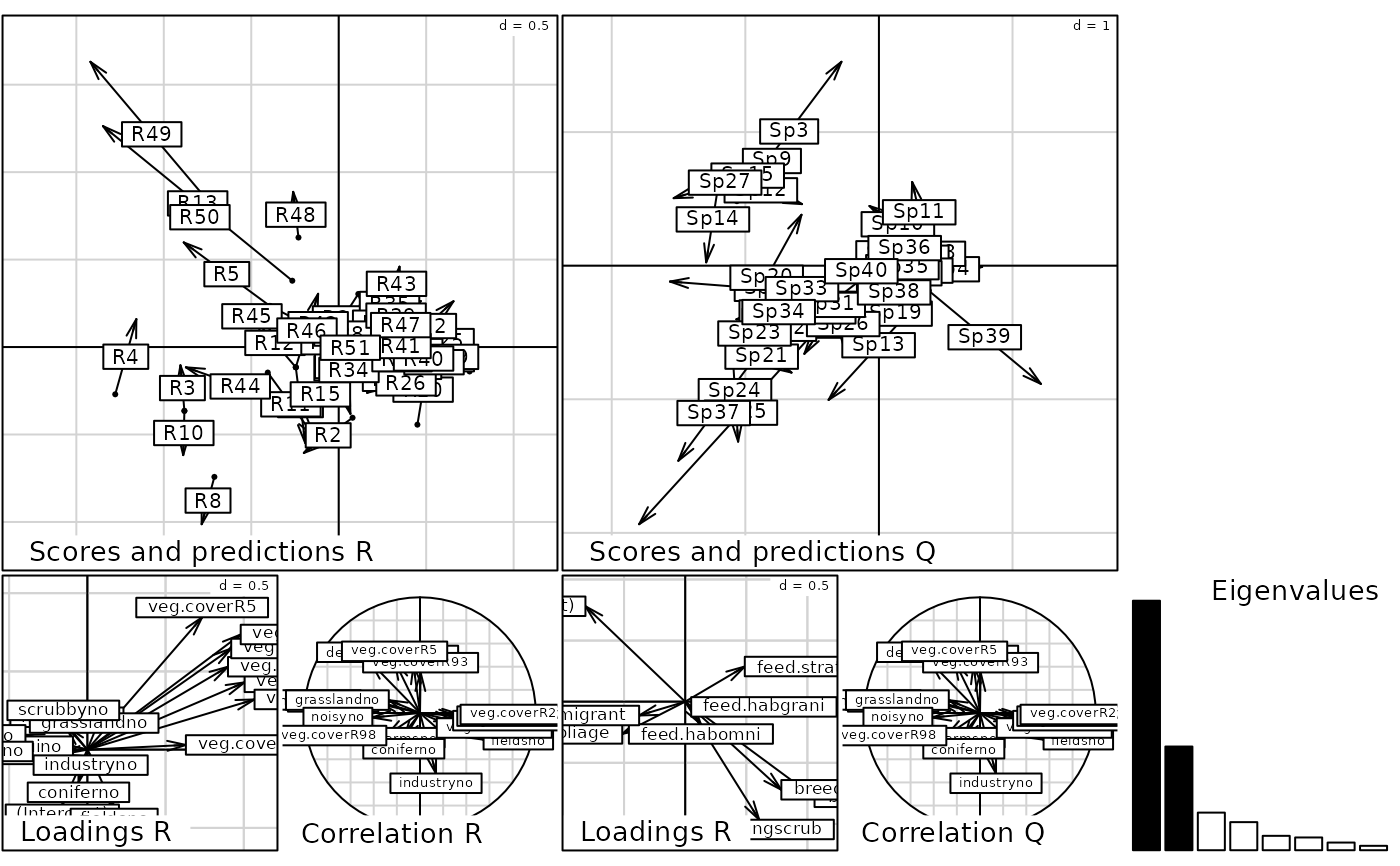
plot(dcca)

randtest(dcca)
#> class: krandtest lightkrandtest 
#> Monte-Carlo tests
#> Call: randtest.dpcaiv(xtest = dcca)
#> 
#> Number of tests:   2 
#> 
#> Adjustment method for multiple comparisons:   none 
#> Permutation number:   99 
#>     Test       Obs  Std.Obs   Alter Pvalue
#> 1 Model2 0.1359425 4.329949 greater   0.01
#> 2 Model4 0.1359425 2.193395 greater   0.02
#> 
dvaripart(coa, aviurba$mil, aviurba$trait, nrepet = 99)
#> Variation Partitioning
#> class: dvaripart list 
#> 
#> Test of fractions:
#> class: krandtest lightkrandtest 
#> Monte-Carlo tests
#> Call: dvaripart(Y = coa, dfR = aviurba$mil, dfQ = aviurba$trait, nrepet = 99)
#> 
#> Number of tests:   4 
#> 
#> Adjustment method for multiple comparisons:   none 
#> Permutation number:   99 
#>          Test       Obs  Std.Obs   Alter Pvalue
#> 1       ab(R) 0.4215783 3.969993 greater   0.01
#> 2       bc(Q) 0.2556643 2.002752 greater   0.02
#> 3 b(RQ)_Rperm 0.1359425 4.476797 greater   0.01
#> 4 b(RQ)_Qperm 0.1359425 2.054284 greater   0.04
#> 
#> 
#> Individual fractions:
#>         a         b         c         d 
#> 0.2856358 0.1359425 0.1197218 0.4586999 
#> 
#> Adjusted fractions:
#>          a          b          c          d 
#> 0.09030311 0.03351889 0.01377559 0.86240242