Small Ecological Dataset

atlas is a list containing three kinds of information about 23 regions (The French Alps) :
geographical coordinates, meteorology and bird presences.

Usage

data(atlas)

Format

atlas is a list of 9 components:

area

is a convex hull of 23 geographical regions.

xy

are the coordinates of the region centers and altitude (in meters).

names.district

is a vector of region names.

meteo

is a data frame with 7 variables: min and max temperature in january; min and max temperature in july; january, july and total rainfalls.

birds

is a data frame with 15 variables (species).

contour

is a data frame with 4 variables (x1, y1, x2, y2) for the contour display of The French Alps.

alti

is a data frame with 3 variables altitude in percentage [0,800], ]800,1500] and ]1500,5000].

Spatial

is the map of the 23 regions of The French Alps (an object of the class SpatialPolygons of sp).

Spatial.contour

is the contour of the map of the 23 regions of the French Alps (an object of the class SpatialPolygons of sp).

Source

Extract from:
Lebreton, Ph. (1977) Les oiseaux nicheurs rhonalpins. Atlas ornithologique Rhone-Alpes. Centre Ornithologique Rhone-Alpes, Universite Lyon 1, 69621 Villeurbanne. Direction de la Protection de la Nature, Ministere de la Qualite de la Vie. 1–354.

Examples

data(atlas)
if(adegraphicsLoaded()) {
  if(requireNamespace("sp", quietly = TRUE)) {
    g11 <- s.Spatial(atlas$Spatial, pSp.col = "white", plot = FALSE)
    g12 <- s.label(atlas$area[, 2:3], plabels.cex = 0, plot = FALSE)
    g1 <- superpose(g11, g12, plot = FALSE)
    g2 <- s.label(atlas$xy, lab = atlas$names.district, Sp = atlas$Spatial, 
      pgrid.dra = FALSE, pSp.col = "white", plot = FALSE)
    obj3 <- sp::SpatialPolygonsDataFrame(Sr = atlas$Spatial, data = atlas$meteo)
    g3 <- s.Spatial(obj3[, 1], nclass = 12, psub = list(position = "topleft", 
      text = "Temp Mini January", cex = 2), plot = FALSE)
    g4 <- s.corcircle((dudi.pca(atlas$meteo, scann = FALSE)$co), plabels.cex = 1, plot = FALSE)
    G1 <- ADEgS(list(g1, g2, g3, g4), layout = c(2, 2))
  
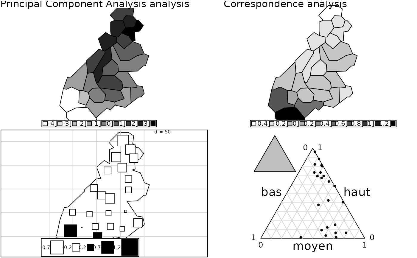
    obj5 <- sp::SpatialPolygonsDataFrame(Sr = atlas$Spatial, 
      data = dudi.pca(atlas$meteo, scann = FALSE)$li)
    g5 <- s.Spatial(obj5[, 1], nclass = 12, psub = list(position = "topleft", 
      text = "Principal Component Analysis analysis", cex = 1.5), plot = FALSE)
    coa1 <- dudi.coa(atlas$birds, scann = FALSE, nf = 1)
    obj6 <- sp::SpatialPolygonsDataFrame(Sr = atlas$Spatial, data = coa1$li)
    g6 <- s.Spatial(obj6[, 1], nclass = 12, psub = list(position = "topleft", 
      text = "Correspondence analysis", cex = 1.5), plot = FALSE)
    g7 <- s.value(atlas$xy, coa1$li$Axis1, Sp = atlas$Spatial.contour, ppoints.cex = 2, 
      porigin.include = FALSE, paxes.draw = FALSE, pSp.col = "white", plot = FALSE)
    g8 <- triangle.label(atlas$alti, plabels.cex = 0, plot = FALSE)
    G2 <- ADEgS(list(g5, g6, g7, g8), layout = c(2, 2))
  
  }
} else {
  op <- par(no.readonly = TRUE) 
  par(mfrow = c(2, 2))
  area.plot(atlas$area, cpoin = 1.5)
  area.plot(atlas$area, lab = atlas$names.district, clab = 1)
  x <- atlas$meteo$mini.jan
  
  names(x) <- row.names(atlas$meteo)
  area.plot(atlas$area, val = x, ncl = 12, sub = "Temp Mini January", csub = 2, cleg = 1)
  s.corcircle((dudi.pca(atlas$meteo, scann = FALSE)$co), clab = 1)
  
  area.plot(atlas$area, val = dudi.pca(atlas$meteo,scann=FALSE)$li[, 1], ncl = 12, 
    sub = "Principal Component Analysis analysis", csub = 1.5, cleg = 1)
  birds.coa <- dudi.coa(atlas$birds, sca = FALSE, nf = 1)
  x <- birds.coa$li$Axis1
  area.plot(atlas$area, val = x, ncl = 12, sub = "Correspondence analysis", csub = 1.5, cleg = 1)
  
  s.value(atlas$xy, x, contour = atlas$contour, csi = 2, incl = FALSE, addax = FALSE)
  triangle.plot(atlas$alti)
  par(op)
  par(mfrow = c(1, 1))}