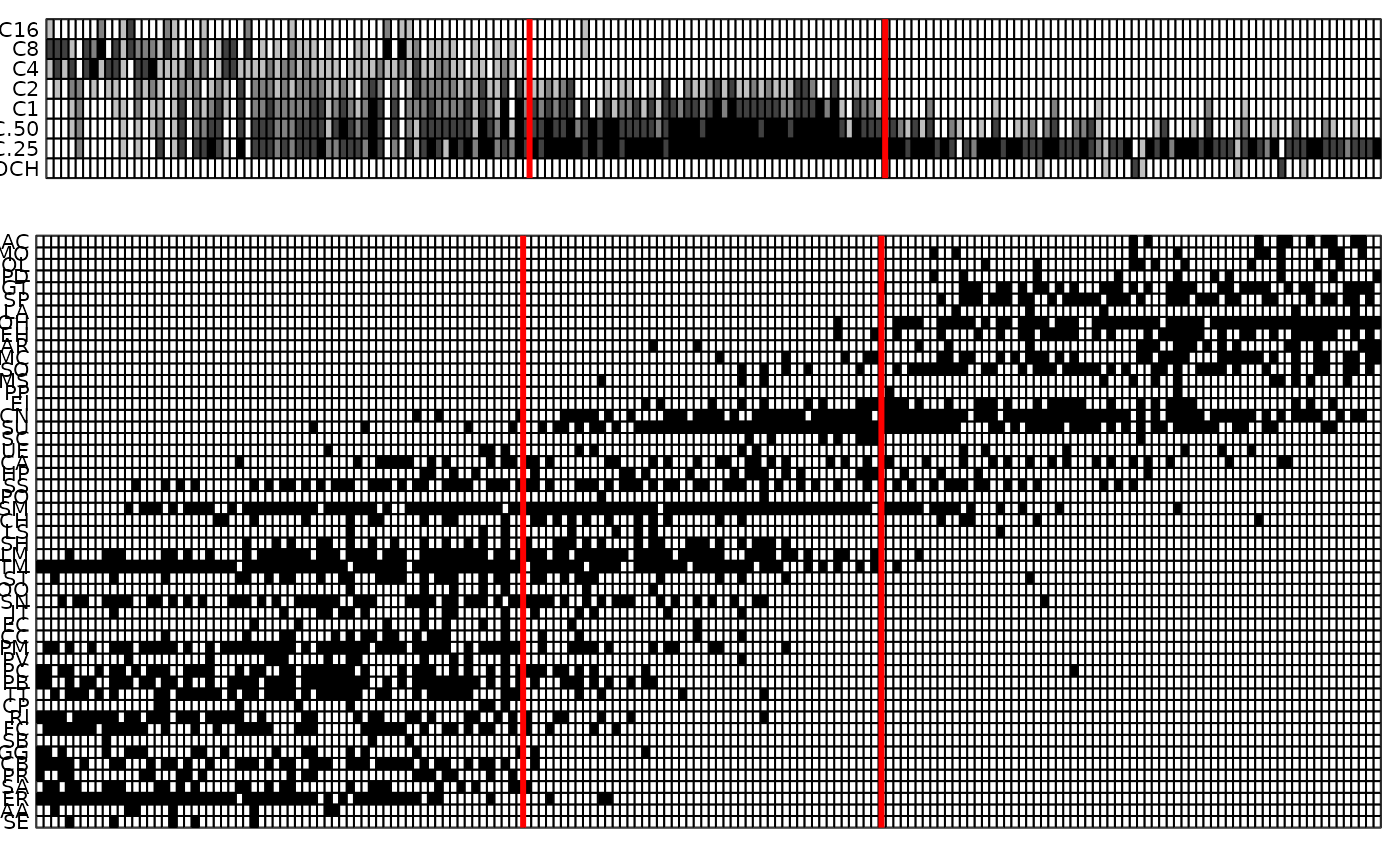
Plot of the arrays by grey levels

presents a graph for viewing the numbers of a table by grey levels.

Usage

table.paint(df, x = 1:ncol(df), y = nrow(df):1, 
    row.labels = row.names(df), col.labels = names(df), 
    clabel.row = 1, clabel.col = 1, csize = 1, clegend = 1)

Arguments

df

a data frame

x

a vector of values to position the columns, used only for the ordered values

y

a vector of values to position the rows, used only for the ordered values

row.labels

a character vector for the row labels

col.labels

a character vector for the column labels

clabel.row

a character size for the row labels

clabel.col

a character size for the column labels

csize

if 'clegend' not NULL, a coefficient for the legend size

clegend

a character size for the legend, otherwise no legend

Author

Daniel Chessel

Examples

data(rpjdl)
X <- data.frame(t(rpjdl$fau))
Y <- data.frame(t(rpjdl$mil))
layout(matrix(c(1,2,2,2,1,2,2,2,1,2,2,2,1,2,2,2), 4, 4))
coa1 <- dudi.coa(X, scan = FALSE)
x <- rank(coa1$co[,1])
y <- rank(coa1$li[,1])
table.paint(Y, x = x, y = 1:8, clabel.c = 0, cleg = 0)
abline(v = 114.9, lwd = 3, col = "red")
abline(v = 66.4, lwd = 3, col = "red")
table.paint(X, x = x, y = y, clabel.c = 0, cleg = 0,
    row.lab = paste("  ", row.names(X), sep = ""))
abline(v = 114.9, lwd = 3, col = "red")
abline(v = 66.4, lwd = 3, col = "red")

par(mfrow = c(1, 1))