Plot of a frequency distribution

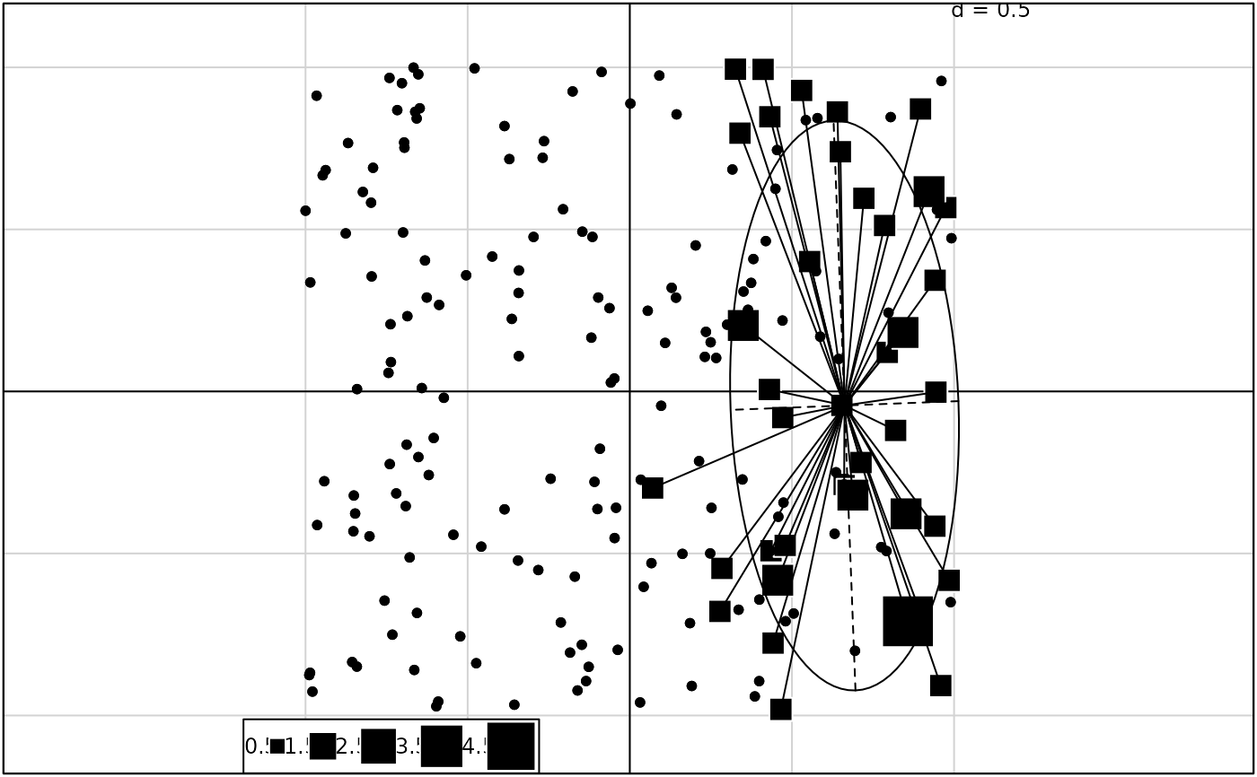
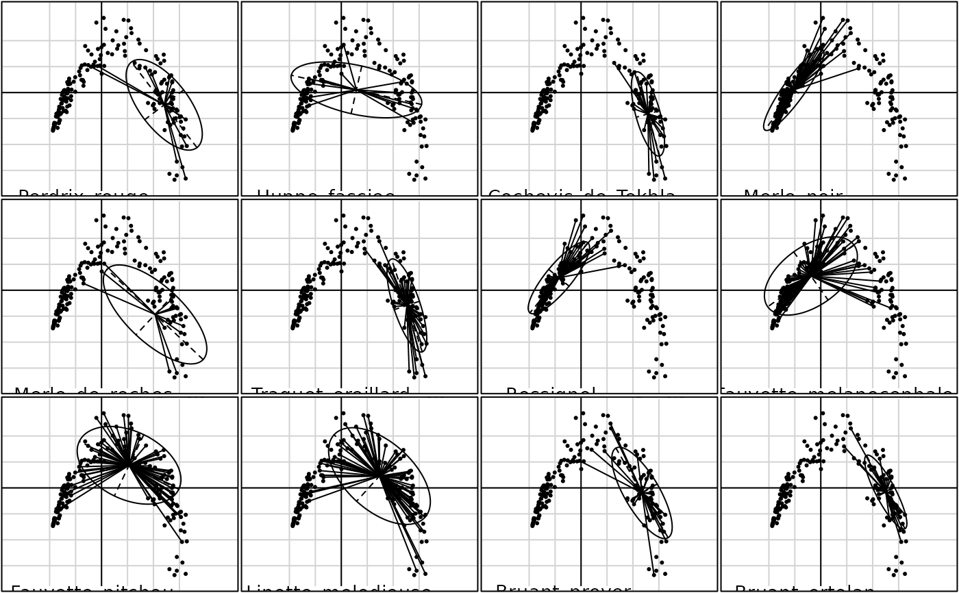
performs the scatter diagram of a frequency distribution.

Usage

s.distri(dfxy, dfdistri, xax = 1, yax = 2, cstar = 1, 
    cellipse = 1.5, axesell = TRUE, label = names(dfdistri), 
    clabel = 0, cpoint = 1, pch = 20, xlim = NULL, ylim = NULL, 
    grid = TRUE, addaxes = TRUE, origin = c(0,0), 
    include.origin = TRUE, sub = "", csub = 1, possub = "bottomleft", 
    cgrid = 1, pixmap = NULL, contour = NULL, area = NULL, add.plot = FALSE)

Arguments

dfxy: a data frame containing two columns for the axes
dfdistri: a data frame containing the mass distributions in columns
xax: the column number for the x-axis
yax: the column number for the y-axis
cstar: a number between 0 and 1 which defines the length of the star size
cellipse: a positive coefficient for the inertia ellipse size
axesell: a logical value indicating whether the ellipse axes should be drawn
label: a vector of strings of characters for the distribution centers labels
clabel: if not NULL, a character size for the labels, used with par("cex")*clabel
cpoint: a character size for plotting the points, used with par("cex")*cpoint. If zero, no points are drawn
pch: if cpoint > 0, an integer specifying the symbol or the single character to be used in plotting points
xlim: the ranges to be encompassed by the x, if NULL they are computed
ylim: the ranges to be encompassed by the y, if NULL they are computed
grid: a logical value indicating whether a grid in the background of the plot should be drawn
addaxes: a logical value indicating whether the axes should be plotted
origin: the fixed point in the graph space, for example c(0,0) the origin axes
include.origin: a logical value indicating whether the point "origin" should be belonged to the graph space
sub: a string of characters to be inserted as legend
csub: a character size for the legend, used with par("cex")*csub
possub: a string of characters indicating the sub-title position ("topleft", "topright", "bottomleft", "bottomright")
cgrid: a character size, parameter used with par("cex")* cgrid to indicate the mesh of the grid
pixmap: an object 'pixmap' displayed in the map background
contour: a data frame with 4 columns to plot the contour of the map : each row gives a segment (x1,y1,x2,y2)
area: a data frame of class 'area' to plot a set of surface units in contour
add.plot: if TRUE uses the current graphics window

Value

The matched call.

Author

Daniel Chessel

Examples

if(!adegraphicsLoaded()) {
  xy <- cbind.data.frame(x = runif(200, -1, 1), y = runif(200, -1, 1))
  distri <- data.frame(w1 = rpois(200, xy$x * (xy$x > 0)))
  s.value(xy, distri$w1, cpoi = 1)
  s.distri(xy, distri, add.p = TRUE)
  
  w1 <- as.numeric((xy$x> 0) & (xy$y > 0))
  w2 <- ((xy$x > 0) & (xy$y < 0)) * (1 - xy$y) * xy$x
  w3 <- ((xy$x < 0) & (xy$y > 0)) * (1 - xy$x) * xy$y
  w4 <- ((xy$x < 0) & (xy$y < 0)) * xy$y * xy$x
  
  distri <- data.frame(a = w1 / sum(w1), b = w2 / sum(w2), 
    c = w3 / sum(w3), d = w4 / sum(w4))
  s.value(xy, unlist(apply(distri, 1, sum)), cleg = 0, csi = 0.75)
  s.distri(xy, distri, clab = 2, add.p = TRUE)
  
  data(rpjdl)
  xy <- dudi.coa(rpjdl$fau, scan = FALSE)$li
  par(mfrow = c(3, 4))
  for (i in c(1, 5, 8, 20, 21, 23, 26, 33, 36, 44, 47, 49)) {
    s.distri(xy, rpjdl$fau[, i], cell = 1.5, sub = rpjdl$frlab[i], 
      csub = 2, cgrid = 1.5)}
  par(mfrow = c(1, 1))
}