Add graphics to an existing plot

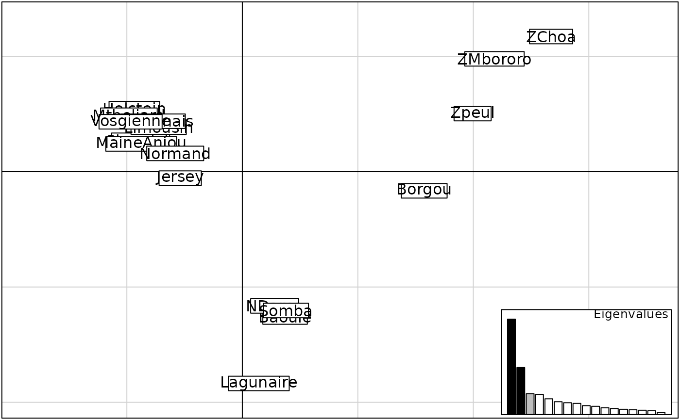
add.scatter is a function which defines a new plot area within an existing plot and displays an additional graphic inside this area. The additional graphic is determined by a function which is the first argument taken by add.scatter. It can be used in various ways, for instance to add a screeplot to an ordination scatterplot (add.scatter.eig).
The function add.scatter.eig uses the following colors: black (represented axes), grey(axes retained in the analysis) and white (others).

Usage

add.scatter(func,posi = c("bottomleft","bottomright","topleft","topright"),
ratio = 0.2, inset = 0.01, bg.col = 'white')
add.scatter.eig(w, nf = NULL, xax, yax, posi = "bottomleft", ratio =
.25, inset = 0.01, sub = "Eigenvalues", csub = 2 * ratio)

Arguments

func

an - evaluated - function producing a graphic

posi

a character vector (only its first element being considered) giving the position of the added graph. Possible values are "bottomleft" (="bottom"),"bottomright","topleft" (="top"),"topright", and "none" (no plot).

ratio

the size of the added graph in proportion of the current plot region

inset

the inset from which the graph is drawn, in proportion of the whole plot region. Can be a vector of length 2, giving the inset in x and y. If atomic, same inset is used in x and y

bg.col

the color of the background of the added graph

w

numeric vector of eigenvalues

nf

the number of retained factors, NULL if not provided

xax

first represented axis

yax

second represented axis

sub

title of the screeplot

csub

size of the screeplot title

Value

The matched call (invisible).

Details

add.scatter uses par("plt") to redefine the new plot region. As stated in par documentation, this produces to (sometimes surprising) interactions with other parameters such as "mar". In particular, such interactions are likely to reset the plot region by default which would cause the additional graphic to take the whole plot region. To avoid such inconvenient, add par([other options], plt=par("plt")) when using par in your graphical function (argument func).

See also

scatter

Author

Thibaut Jombart t.jombart@imperial.ac.uk

Examples

  data(microsatt)
  w <- dudi.coa(data.frame(t(microsatt$tab)), scann = FALSE, nf = 3)
    
  if(adegraphicsLoaded()) {
    a1 <- rnorm(100)
    b1 <- s1d.barchart(sort(a1), p1d.horizontal = FALSE, plot = FALSE)
    h1 <- s1d.hist(a1, pgrid.draw = FALSE, porigin.draw = FALSE, pbackground.col = "grey", 
      plot = FALSE, ppoly.col = "white", ppoly.alpha = 1)
    g1 <- insert(h1, b1, posi = "topleft", plot = FALSE)
  
    a2 <- rnorm(100)
    b2 <- s1d.barchart(sort(a2), p1d.horizontal = FALSE, plot = FALSE)
    h2 <- s1d.hist(a2, pgrid.draw = FALSE, porigin.draw = FALSE, pbackground.col = "grey", 
      plot = FALSE, ppoly.col = "white", ppoly.alpha = 1)
    g2 <- insert(h2, b2, posi = "topleft", inset = c(0.25, 0.01), plot = FALSE)
  
    a3 <- rnorm(100)
    b3 <- s1d.barchart(sort(a3), p1d.horizontal = FALSE, plot = FALSE)
    h3 <- s1d.hist(a3, pgrid.draw = FALSE, porigin.draw = FALSE, pbackground.col = "grey", 
      plot = FALSE, ppoly.col = "white", ppoly.alpha = 1)
    g3 <- insert(h3, b3, posi = "bottomleft", inset = 0.4, ratio = 0.2, plot = FALSE)
  
    a4 <- rnorm(100)
    b4 <- s1d.barchart(sort(a4), p1d.horizontal = FALSE, plot = FALSE)
    h4 <- s1d.hist(a4, pgrid.draw = FALSE, porigin.draw = FALSE, pbackground.col = "grey", 
      plot = FALSE, ppoly.col = "white", ppoly.alpha = 1)
    g4 <- insert(h3, b3, posi = "bottomright", ratio = 0.3, plot = FALSE)
    
    G1 <- ADEgS(list(g1, g2, g3, g4), layout = c(2, 2), plot = TRUE)
    
    g5 <- s.label(w$co, plot = FALSE)
    g6 <- plotEig(w$eig, w$nf, psub = list(text = "Eigenvalues"), 
      pbackground = list(box = TRUE), plot = FALSE)
    G2 <- insert(g6, g5, posi = "bottomright", ratio = 0.25)

  } else {
    par(mfrow=c(2,2))
    f1 <- function(a){
      opar=par("mar","xaxt","yaxt","plt")
      on.exit(par(opar))
      par(mar=rep(.1,4),xaxt="n",yaxt="n",plt=par("plt"))
    
      hist(a,xlab="",ylab="",main="",col="white",proba=TRUE)
      lines(seq(-4,4,le=50),dnorm(seq(-4,4,le=50)),col="red")
    }
    
    a <- rnorm(100)
    barplot(sort(a))
    add.scatter(f1(a),posi="topleft",bg.col="grey")
    
    a <- rnorm(100)
    barplot(sort(a))
    add.scatter(f1(a),posi="topleft",bg.col="grey",inset=c(.25,.01))
    
    a <- rnorm(100)
    barplot(sort(a))
    add.scatter(f1(a),posi="topleft",bg.col="grey",inset=.25,ratio=.1)
    
    a <- rnorm(100)
    barplot(sort(a))
    add.scatter(f1(a),posi="bottomright",bg.col="grey",ratio=.3)
    par(mfrow=c(1,1))
    
    s.label(w$co)
    add.scatter.eig(w$eig,w$nf,posi="bottomright",1,2)
  }