Electoral Data
elec88.RdThis data set gives the results of the presidential election in France in 1988 for each department and all the candidates.
Usage
data(elec88)Format
elec88 is a list with the following components:
- tab
a data frame with 94 rows (departments) and 9 variables (candidates)
- res
the global result of the election all-over the country
- lab
a data frame with two variables:
elec88$lab$depis a vector containing the names of the 94 french departments,elec88$lab$regis a vector containing the names of the 21 French administrative regions.- area
the data frame of 3 variables returning the boundary lines of each department. The first variable is a factor. The levels of this one are the row.names of
tab. The second and third variables return the coordinates (x, y) of the points of the boundary line.- contour
a data frame with 4 variables (x1, y1, x2, y2) for the contour display of France
- xy
a data frame with two variables (x, y) giving the position of the center for each department
- nb
the neighbouring graph between departments, object of the class
nb- Spatial
the map of the french departments in Lambert II coordinates (an object of the class
SpatialPolygonsofsp)- Spatial.contour
the contour of the map of France in Lambert II coordinates (an object of the class
SpatialPolygonsofsp)
Examples
data(elec88)
apply(elec88$tab, 2, mean)
#>  Mitterand     Chirac      Barre     Le.Pen   Lajoinie   Waechter     Juquin
#> 34.3063830 20.2670213 16.4680851 13.7606383  6.7106383  3.8638298  2.1670213
#> Laguillier    Boussel
#>  2.0574468  0.3989362
summary(elec88$res)
#>    Min. 1st Qu.  Median    Mean 3rd Qu.    Max.
#>    0.40    2.10    6.80   11.11   16.50   34.10
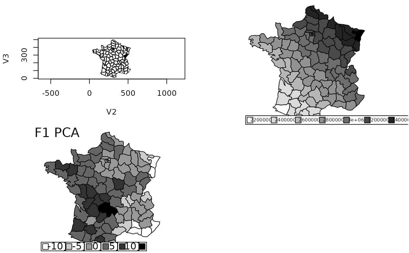
pca1 <- dudi.pca(elec88$tab, scale = FALSE, scannf = FALSE)

if(adegraphicsLoaded()) {
  if(requireNamespace("sp", quietly = TRUE)) {
    data1 <- as.data.frame(as.numeric(rownames(elec88$tab) == "D25"))
    rownames(data1) <- row.names(elec88$Spatial)
    obj1 <- sp::SpatialPolygonsDataFrame(Sr = elec88$Spatial, data = data1)
    g1 <- s.Spatial(obj1, psub.text = "", plot = FALSE)
    g2 <- s.Spatial(obj1, psub.text = "", nb = elec88$nb, pnb.node.cex = 0, plot = FALSE)

    data3 <- as.data.frame(elec88$xy[, 1] + elec88$xy[, 2])
    rownames(data3) <- row.names(elec88$Spatial)
    obj3 <- sp::SpatialPolygonsDataFrame(Sr = elec88$Spatial, data = data3)
    g3 <- s.Spatial(obj3, psub.text = "", plot = FALSE)

    data4 <- as.data.frame(pca1$li[, 1])
    rownames(data4) <- row.names(elec88$Spatial)
    obj4 <- sp::SpatialPolygonsDataFrame(Sr = elec88$Spatial, data = data4)
    g4 <- s.Spatial(obj4, psub.text = "F1 PCA", plot = FALSE)

    G <- ADEgS(list(g1, g2, g3, g4), layout = c(2, 2))
  }

} else {
  par(mfrow = c(2, 2))
  plot(elec88$area[, 2:3], type = "n", asp = 1)
  lpoly <- split(elec88$area[, 2:3], elec88$area[, 1])
  lapply(lpoly, function(x) {points(x, type = "l"); invisible()})
  polygon(elec88$area[elec88$area$V1 == "D25", 2:3], col = 1)
  area.plot(elec88$area, val = elec88$xy[, 1] + elec88$xy[, 2])
  area.plot(elec88$area, val = pca1$li[, 1], sub = "F1 PCA",
    csub = 2, cleg = 1.5)
  par(mfrow = c(1, 1))
}
