Maximal value of Rao's diversity coefficient also called quadratic entropy

For a given dissimilarity matrix, this function calculates the maximal value of Rao's diversity coefficient over all frequency distribution. It uses an optimization technique based on Rosen's projection gradient algorithm and is verified using the Kuhn-Tucker conditions.

Usage

divcmax(dis, epsilon, comment)

Arguments

dis: an object of class dist containing distances or dissimilarities among elements.
epsilon: a tolerance threshold : a frequency is non null if it is higher than epsilon.
comment: a logical value indicating whether or not comments on the optimization technique should be printed.

Value

Returns a list

value: the maximal value of Rao's diversity coefficient.
vectors: a data frame containing four frequency distributions : sim is a simple distribution which is equal to \(\frac{D1}{1^tD1}\), pro is equal to \(\frac{z}{1^tz1}\), where z is the nonnegative eigenvector of the matrix containing the squared dissimilarities among the elements, met is equal to \(z^2\), num is a frequency vector maximizing Rao's diversity coefficient.

References

Rao, C.R. (1982) Diversity and dissimilarity coefficients: a unified approach. Theoretical Population Biology, 21, 24–43.

Gini, C. (1912) Variabilità e mutabilità. Universite di Cagliari III, Parte II.

Simpson, E.H. (1949) Measurement of diversity. Nature, 163, 688.

Champely, S. and Chessel, D. (2002) Measuring biological diversity using Euclidean metrics. Environmental and Ecological Statistics, 9, 167–177.

Pavoine, S., Ollier, S. and Pontier, D. (2005) Measuring diversity from dissimilarities with Rao's quadratic entropy: are any dissimilarities suitable? Theoretical Population Biology, 67, 231–239.

Author

Stéphane Champely Stephane.Champely@univ-lyon1.fr
Sandrine Pavoine pavoine@mnhn.fr

Examples

data(elec88)

# Dissimilarity matrix.
d0 <- dist(elec88$xy/100)

# Frequency distribution maximizing spatial diversity in France
# according to Rao's quadratic entropy.
France.m <- divcmax(d0)
w0 <- France.m$vectors$num
v0 <- France.m$value
idx <- (1:94) [w0 > 0]

if(!adegraphicsLoaded()) {
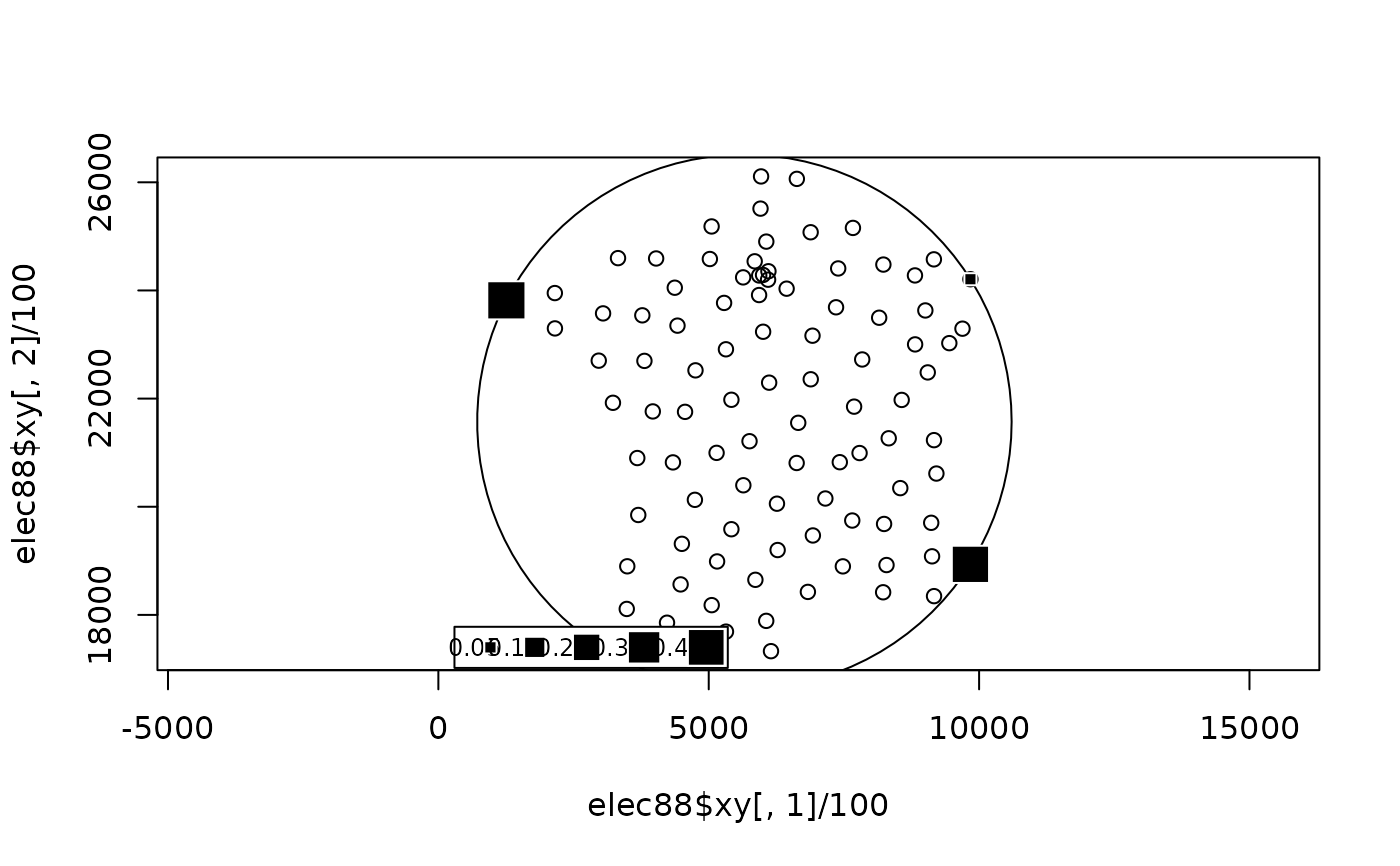
  # Smallest circle including all the 94 departments.
  # The squared radius of that circle is the maximal value of the
  # spatial diversity.
  w1 <- elec88$xy[idx, ]/100
  w.c <- apply(w1 * w0[idx], 2, sum)
  plot(elec88$xy[, 1]/100, elec88$xy[, 2]/100, asp=1)
  symbols(w.c[1], w.c[2], circles = sqrt(v0), inches = FALSE, add = TRUE)
  s.value(elec88$xy/100, w0, add.plot = TRUE)
}