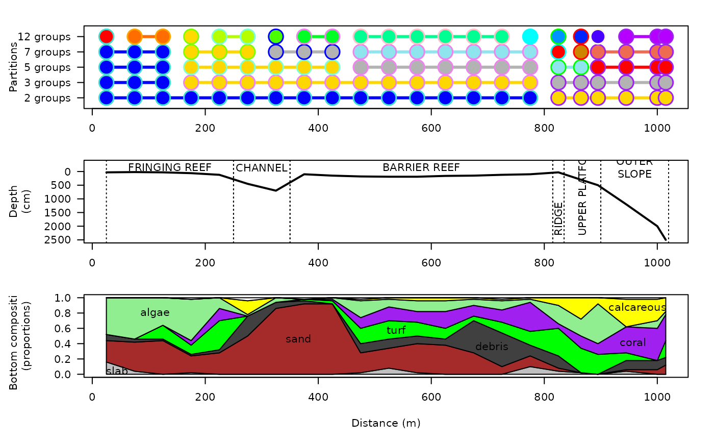
Tiahura Transect Fish Data Set — Tiahura • adespatial

Fish community composition, ecological traits, and environmental characteristics observed along a 1-km coral reef transect.

data(Tiahura)

Format

A list with four elements:

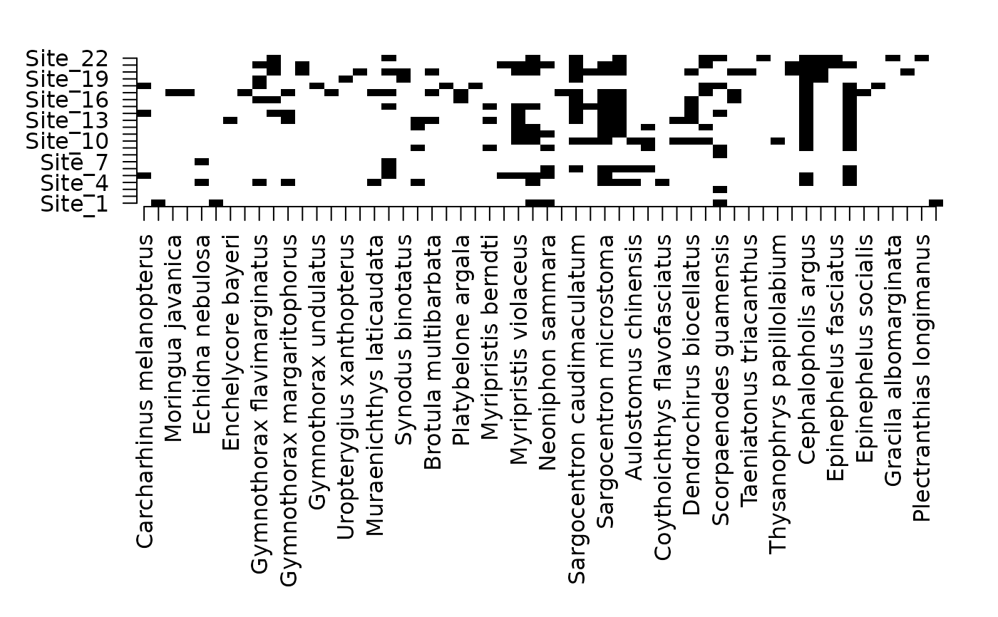
fish: A data frame with 22 rows (sites) and 280 columns (fish species) describing the presence (value: 1) or absence (value: 0) of the fish species at the sites.
species: A character vector with 280 elements containing the binomial (latin) names of the 280 fish species.
trait: A data frame with 280 rows (species) and five columns (traits) containing the species ecological traits (see details).
habitat: A data frame with 22 rows (sites) and 10 columns (characteristics) containing the environmental characteristics of the sites (see details).
reef: A data frame with 6 rows (sections) and 3 columns describing the different sections of the transect (see details).

Source

Pierre Legendre <pierre.legendre@umontreal.ca>, René Galzin <pol@univ-perp.fr>, Mireille Harmelin-Vivien <Harmelin@com.univ-mrs.fr>, and Guillaume Guenard <guillaume.guenard@gmail.com>

Details

The Tiahura fish transect data was described and analyzed by Galzin & Legendre (1987). It consists of presence/absence data for 280 fish species observed at $22$ sites along a 1.02 km long coast-to-sea cross-reef transect located near the northwestern corner of the high volcanic island of Moorea (French Polynesia; WGS84: -17.4934, -149.8680). The survey sites were 50 m long. Species presence/absence data were recorded by a diver trained in underwater fish identification. The transect began on a coral sand beach, followed by a zone of detritic sediments, then a dying reef flat, followed by a zone of coral patches. That relatively flat area ended at a 100-m wide - 9-m deep channel, followed by a 490-m wide barrier reef, which ended in a slightly elevated reef ridge, followed by the outer slope into the Pacific Ocean. The survey was terminated at depth of approximately 25 m; this is the maximum depth allowing scuba diving for any length of time without having to perform decompression stops. For further details about the transect and survey method, see Galzin & Legendre (1987).

Ecological traits contained in data frame trait are

Feeding: A seven-level categorical variables describing the feeding habits of the fish species
Ecology: A seven-level categorical variable describing the general behavior of the fish species in their habitats
Adult: A six-level ordered variables describing the adult sizes of the fish species
Egg: A three-level categorical variable describing the types of eggs laid by the fish species
Activity: A three-level categorical variable describing the activity rhythm of the fish species

Environmental characteristics contained in data frame habitat are the distance from the shore (in m), the water depth at the site (in cm), and substrate composition. Substrate composition (environmental characteristics 3 - 10) is described by percentage coverage indices of the reef bottom by different materials, based on 50 observation points. These observations points were positioned at 1-m intervals along a 50-m rope. The variables indicate what proportion of the 50 readings pertained to each category of substrate. Several of these categories represent biological materials lying on top of, intermingled with, or attached to the mineral substrate. When the 22 stations are considered globally, these eight substrate categories respectively represent 2.5 0.7

Data frame reef, which contains the boundaries of the different sections of the transect, comes in handy for displaying data graphically and interpret results.

This data set was made available to the students in the European Advanced Course "Numerical Analysis in Marine Ecology" given at Observatoire océanologique, Université Paris VI, Villefranche-sur-Mer, on 3 - 20 July 1996.

References

Galzin, R. & P. Legendre. 1987. The fish communities of a coral reef transect. Pacific Science 41: 158-165.

Legendre, P., R. Galzin & M. Harmelin-Vivien. 1997. Relating behavior to habitat: Solutions to the fourth-corner problem. Ecology 78: 547-562

Examples

data(Tiahura)

## Compute dissimilary matrix from Jaccard's similarity coefficient:
tiah.jac <- dist.ldc(Tiahura$fish,method = "jaccard")
#> Info -- D is Euclidean because the function outputs D[jk] = sqrt(1-S[jk])

## Constrained clustering of the fish species:
tiah.chclust <- constr.hclust(tiah.jac, coords=Tiahura$habitat[,"distance"],
                              chron=TRUE)

## Plotting the results
par(mfrow=c(3,1))

## First graph: constrained clusters
par(mar=c(3,6.5,2,2))
dst <- Tiahura$habitat[,"distance"]
plot(NA, xlim=range(dst), ylim=c(0.5,5.5), yaxt="n",
     ylab="Partitions\n\n", xlab="")
parts <- c(2,3,5,7,12)
cols <- c("turquoise", "orange", "chartreuse", "aquamarine", "blue",
          "violet", "pink", "cyan", "green", "red", "cornsilk", "purple")
for(i in 1L:length(parts)) {
  tiah.chclust$coords[,"y"] <- i
  plot(tiah.chclust, parts[i], link=TRUE, lwd=3, hybrids="none",
       lwd.pt=0.5, cex=3, pch=21, plot=FALSE,
       col=cols[round(seq(1,length(cols), length.out=parts[i]))])
}
axis(2, at=1:length(parts), labels=paste(parts,"groups"), las=1)

## Second graph: transect profile
par(mar=c(4,6.5,1,2))
plot(x=dst, y=Tiahura$habitat[,"depth"],
     ylim=c(max(range(Tiahura$habitat[,"depth"])),-300),
     las=1, ylab="Depth\n(cm)\n", xlab="", type="l", lwd=2)
for(i in 1:nrow(Tiahura$reef)) {
  abline(v=Tiahura$reef[i,2], lty=3)
  abline(v=Tiahura$reef[i,3], lty=3)
  if((Tiahura$reef[i,3] - Tiahura$reef[i,2])<100) {
    text(x=(Tiahura$reef[i,2] + Tiahura$reef[i,3])/2, y=2350,
         labels=toupper(Tiahura$reef[i,1]),srt=90,adj=0)
  } else {
    text(x=(Tiahura$reef[i,2] + Tiahura$reef[i,3])/2, y=-150,
         labels=toupper(Tiahura$reef[i,1]))
  }
}

## Third graph: bottom composition
par(mar=c(5,6.5,0,2))
plot(NA,xlim=range(dst), ylim=c(0,1), las=1,
     ylab="Bottom composition\n(proportions)\n", xlab="Distance (m)")
bot <- cbind(0, Tiahura$habitat[,3:10])
for(i in 2:9) bot[,i] <- bot[,i] + bot[,i-1]
cols <- c("", "grey75", "brown", "grey25", "green", "purple",
          "lightgreen", "yellow", "white")
for(i in 2:9)
  polygon(x=c(dst, rev(dst)),y=c(bot[,i], rev(bot[,i-1]))/50,
          col=cols[i])
text(x=c(44, 365, 707, 538, 957, 111, 965),
     y=c(0.05, 0.47, 0.37, 0.58, 0.42, 0.80, 0.88),
     labels=colnames(bot)[2:8], xpd=TRUE)


## Species presence graph set:
plot_slice <- function(sl,split) {
  size <- ceiling(length(Tiahura$species)/split)
  sp_slice <- size*(sl - 1L) + (1L:size)
  image(z=t(as.matrix(Tiahura$fish[,sp_slice])),y=1:nrow(Tiahura$fish),
        x=1:length(sp_slice),zlim=c(0,1),col=c("white","black"),axes=FALSE,
        ylab="",xlab="")
  axis(1L,at=1:length(sp_slice),labels=Tiahura$species[sp_slice],las=2L)
  axis(2L,at=1:nrow(Tiahura$fish),label=rownames(Tiahura$fish),las=1L)
  invisible(NULL)
}

par(mar=c(15,5,2,2))
plot_slice(1L,5L)
#> Error in plot.new(): figure margins too large
## plot_slice(2L,5L)
## plot_slice(3L,5L)
## plot_slice(4L,5L)
## plot_slice(5L,5L)