Space- And Time-Constrained Clustering

Function constr.hclust carries out space-constrained or time-constrained agglomerative clustering from a multivariate dissimilarity matrix.

constr.hclust(
  d,
  method = "ward.D2",
  links,
  coords,
  beta = -0.25,
  chron = FALSE,
  members = NULL
)

Arguments

d: A dist-class dissimilarity (distance) matrix.
method: The agglomeration method to be used (default: "ward.D2"; see details).
links: A list of edges (or links) connecting the points. May be omitted in some cases; see details and examples
coords: Coordinates of the observations (data rows) in the dissimilarity matrix d. The coordinates are used for plotting maps of the clustering results. This matrix may be omitted when the user does not wish to print maps of the clustering results or when no links file is provided. coords is a matrix or data frame with two columns, following the convention of the Cartesian plane: first column for abscissa, second column for ordinate. See examples.
beta: The beta parameter for beta-flexible clustering (default: beta = -0.25).
chron: Logical (TRUE or FALSE) indicating whether a chronological (i.e. time-constrained or spatial transect) clustering should be calculated (default: chron = FALSE).
members: NULL or a vector with length size of d (default: NULL; See details).

Value

A constr.hclust-class object.

Details

The agglomeration method to be used should be (an unambiguous abbreviation of) one of "ward.D", "ward.D2", "single", "complete", "average" (UPGMA), "mcquitty" (WPGMA), "centroid" (UPGMC), "median" (WPGMC), or "flexible". Method "ward.D2" (default) implements the Ward (1963) clustering criterion, method "ward.D" does not (Murtagh and Legendre, 2014).

Agglomerative clustering can be carried out with a constraint of spatial or temporal contiguity. This means that only the objects that are linked in links are considered to be candidates for clustering: the next pair of objects to cluster will be the pair that has the lowest dissimilarity value among the pairs that are linked.

The same rule applies during the subsequent clustering steps, which involve groups of objects: the list of links is updated after each agglomeration step. All objects that are neighbours of one of the components that have fused are now neighbours of the newly formed cluster.

The edges (links) are specified using argument links, which can be an object of class nb (see, e.g., tri2nb), an object of class listw (see, e.g., nb2listw), a two-element list or an object coercible as a such (e.g., a two-column dataframe), or a two-column matrix with each row representing an edge and the columns representing the two ends of the edges. For lists with more than two elements, as well as dataframes or matrices with more than two-columns, only the first two elements or columns are used for the analysis. The edges are interpreted as being non directional; there is no need to specify an edge going from point a to point b and one going from point b to point a. While doing so is generally inconsequential for the analysis, it carries some penalty in terms of computation time. It is a good practice to place the nodes in increasing order of numbers from the top to the bottom and from the left to the right of the list but this is not mandatory. A word of caution: in cases where clusters with identical minimum distances occur, the order of the edges in the list may have an influence on the result. Alternative results would be statistically equivalent.

When argument link is omitted, regular (unconstrained) clustering is performed and a hclust-class object is returned unless argument chron = TRUE. When argument chron = TRUE, chronological clustering is performed, taking the order of observations as their positions in the sequence. Argument links is not used when chron = TRUE. Argument chron allows one to perform a chronological clustering in the case where observations are ordered chronologically. Here, the term "chronologically" should not be taken restrictively: the method remains applicable to other sequential data sets such as spatial series made of observations along a transect.

When the graph described by link is not entirely connected, a warning message is issued to warn the user about the presence and number of disjoint clusters and a procedure is suggested to identify the disjoint clusters. The disjoint clusters (or singletons) are merged in the order of their indices (i.e. the two clusters with smallest indices are merged first) and so on until all of disjoint clusters have been merged. The dissimilarity at which these clusters are merged is a missing value (NA) in vector height (i.e., unconnected clusters have undefined dissimilarities in constrained clustering).

If members != NULL, then d is taken to be a dissimilarity matrix between clusters instead of dissimilarities between individual objects. Then, members must be a vector giving the number of observations per cluster. In this way, the hierarchical clustering algorithm can be ‘started in the middle of the dendrogram’, e.g., in order to reconstruct the part of the tree above a cut. See examples in hclust for details on that functionality."

Memory storage and time to compute constrained clustering for N objects. The Lance and Williams algorithm for agglomerative clustering uses dissimilarity matrices. The amount of memory needed to store the dissimilarities among N observations as 64-bit double precision floating point variables (IEEE 754) is 8*N*(N-1)/2 bytes. For example, a dissimilarity matrix among 22 500 observations would require 2 024 910 000 bytes (1.89 GiB) of storage whereas one among 100 000 observations would take up 39 999 600 000 bytes (37.25 GiB). The implementation in this function needs to cache a copy of the dissimilarity matrix as its elements are modified following each merging of the closest clusters or singletons, thereby doubling the amounts of required memory shown above. Memory needed to store the other information associated with the clustering is much smaller. Users should make sure to have the necessary memory space (and system stability) before attempting to analyze large data sets. What is considered a large amount of memory has increased over time as computer hardware evolved with time. We let users apply contemporary common sense as to what sample sizes represent manageable clustering problems. Computation time grows with N at roughly the same speed as memory storage requirement to store the dissimilarity matrices increases. See the Benchmarking example below.

With large data sets, a manageable output describing the classification of the sites is obtained with function cutree(x, k) where k is the number of groups. A dendrogram would be unreadable.

References

Guénard, G. and P. Legendre. 2022. Hierarchical clustering with contiguity constraint in R. Journal of Statistical Software 103(7): 1-26 doi:10.18637/jss.v103.i07

Langfelder, P. and S. Horvath. 2012. Fast R functions for robust correlations and hierarchical clustering. Journal of Statistical Software 46(11): 1-17. doi:10.18637/jss.v046.i11

Legendre, P. and L. Legendre. 2012. Numerical ecology, 3rd English edition. Elsevier Science BV, Amsterdam. doi:10.1016/S0304-3800(00)00291-X

Murtagh, F. and P. Legendre. 2014. Ward’s hierarchical agglomerative clustering method: which algorithms implement Ward’s criterion? Journal of Classification 31: 274-295. doi:10.1007/s00357-014-9161-z

Ward, J. H. 1963. Hierarchical grouping to optimize an objective function. Journal of the American Statistical Association 58: 236-244. doi:10.1080/01621459.1963.10500845

Author

Pierre Legendre pierre.legendre@umontreal.ca (preliminary version coded in R) and Guillaume Guénard guillaume.guenard@umontreal.ca (present version mostly coded in C)

Examples


## First example: Artificial map data from Legendre & Legendre
##                (2012, Fig. 13.26): n = 16

dat <- c(41,42,25,38,50,30,41,43,43,41,30,50,38,25,42,41)
coord.dat <- matrix(c(1,3,5,7,2,4,6,8,1,3,5,7,2,4,6,8,
                      4.4,4.4,4.4,4.4,3.3,3.3,3.3,3.3,
                      2.2,2.2,2.2,2.2,1.1,1.1,1.1,1.1),16,2)

## Obtaining a list of neighbours:
library(spdep)
listW <- nb2listw(tri2nb(coord.dat), style="B")
links.mat.dat <- listw2mat(listW)
neighbors <- listw2sn(listW)[,1:2]

## Calculating the (Euclidean) distance between points:
D.dat <- dist(dat)

## Display the points:
plot(coord.dat, type='n',asp=1)
title("Delaunay triangulation")
text(coord.dat, labels=as.character(as.matrix(dat)), pos=3)
for(i in 1:nrow(neighbors))
    lines(rbind(coord.dat[neighbors[i,1],],
          coord.dat[neighbors[i,2],]))


## Unconstrained clustring by hclust:
grpWD2_hclust <- hclust(D.dat, method="ward.D2")
plot(grpWD2_hclust, hang=-1)


## Clustering without a contiguity constraint;
## the result is represented as a dendrogram:
grpWD2_constr_hclust <- constr.hclust(D.dat, method="ward.D2")
plot(grpWD2_constr_hclust, hang=-1)


## Clustering with a contiguity constraint described by a list of
## links:
grpWD2cst_constr_hclust <-
    constr.hclust(
        D.dat, method="ward.D2",
        neighbors, coord.dat)

## To visualize using hclust's plotting method:
## stats:::plot.hclust(grpWD2cst_constr_hclust, hang=-1)

## Plot the results on a map with k=3 clusters:
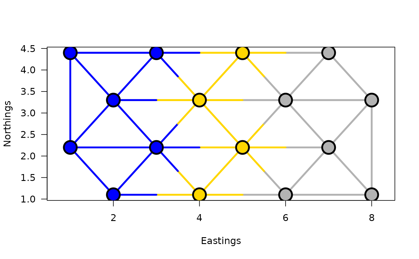
plot(grpWD2cst_constr_hclust, k=3, links=TRUE, las=1, xlab="Eastings",
     ylab="Northings", cex=3, lwd=3)


## Generic functions from hclust can be used, for instance to obtain
## a list of members of each cluster:
cutree(grpWD2cst_constr_hclust, k=3)
#>  [1] 1 1 2 3 1 2 3 3 1 1 2 3 1 2 3 3

## Now with k=5 clusters:
plot(grpWD2cst_constr_hclust, k=5, links=TRUE, las=1, xlab="Eastings",
     ylab="Northings", cex=3, lwd=3)

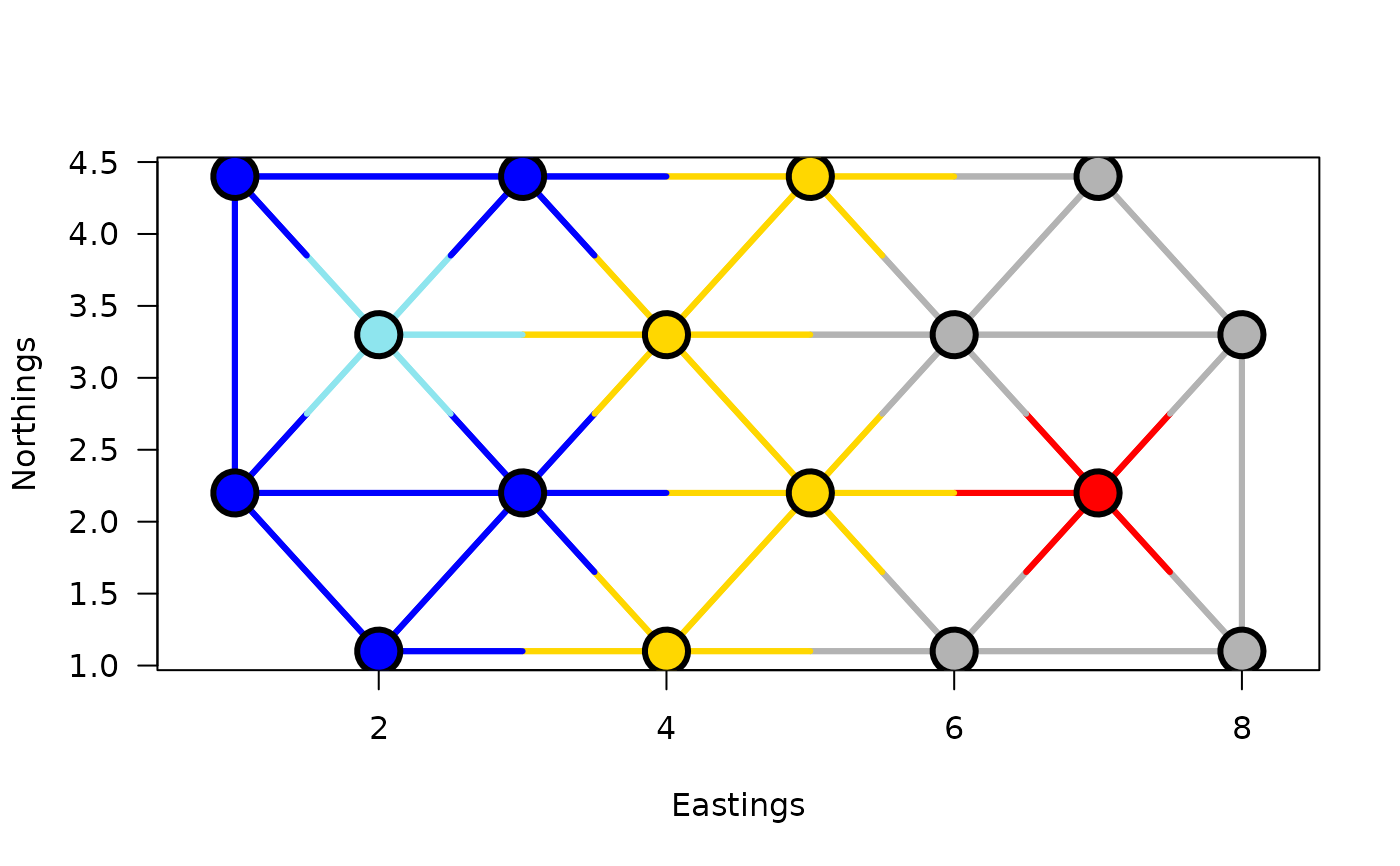cutree(grpWD2cst_constr_hclust, k=5)
#>  [1] 1 1 2 3 4 2 3 3 1 1 2 5 1 2 3 3

## End of the artificial map example


## Second example: Scotch Whiskey distilleries clustered using tasting
## scores (nose, body, palate, finish, and the four distances combined)
## constrained with respect to the distillery locations in Scotland.

## Documentation file about the Scotch Whiskey data: ?ScotchWhiskey

data(ScotchWhiskey)

## Cluster analyses for the nose, body, palate, and finish D
## matrices:

grpWD2cst_ScotchWhiskey <-
    lapply(
        ScotchWhiskey$dist,    ## A list of distance matrices
        constr.hclust,         ## The function called by function lapply
        links=ScotchWhiskey$neighbors@data,         ## The list of links
        coords=ScotchWhiskey$geo@coords/1000
    )

## The four D matrices (nose, body, palate, finish), represented as
## vectors in the ScotchWiskey data file, are combined as follows to
## produce a single distance matrix integrating all four types of
## tastes:

Dmat <- ScotchWhiskey$dist
ScotchWhiskey[["norm"]] <-
    sqrt(Dmat$nose^2 + Dmat$body^2 + Dmat$palate^2 + Dmat$finish^2)

## This example shows how to apply const.clust to a single D matrix when
## the data file contains several matrices.

grpWD2cst_ScotchWhiskey[["norm"]] <-
    constr.hclust(
        d=ScotchWhiskey[["norm"]],method="ward.D2",
        ScotchWhiskey$neighbors@data,
        coords=ScotchWhiskey$geo@coords/1000
    )

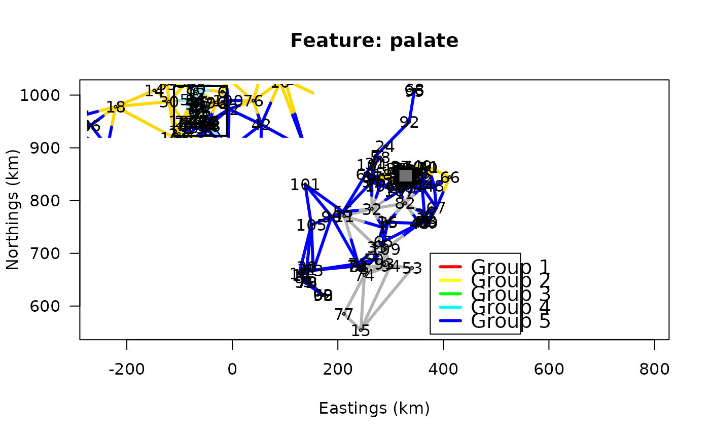
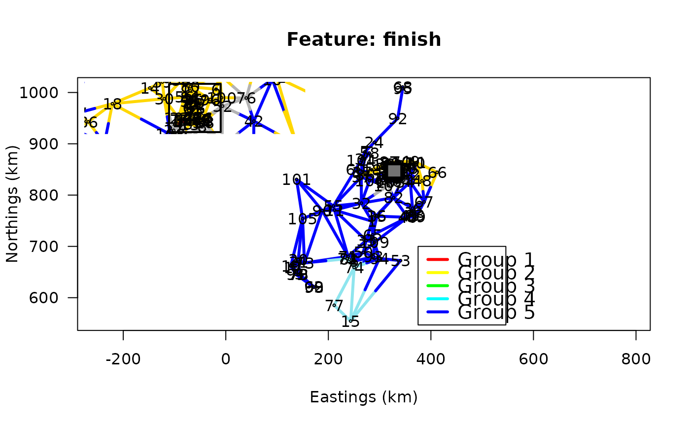
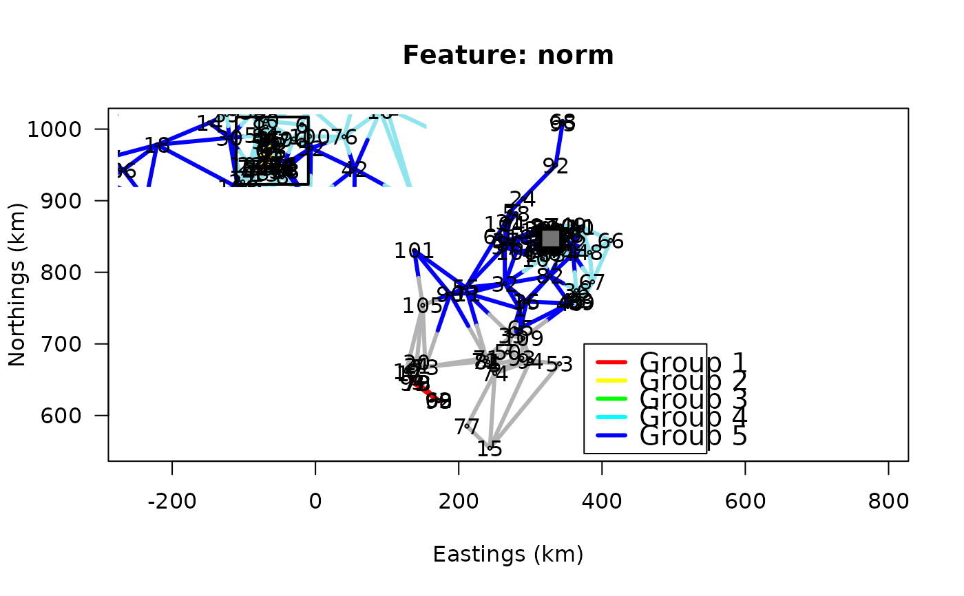
## A fonction to plot the Whiskey clustering results:

plotWhiskey <- function(wh, k) {
   par(fig=c(0,1,0,1))
   plot(grpWD2cst_ScotchWhiskey[[wh]], k=k, links=TRUE, las=1,
        xlab="Eastings (km)", ylab="Northings (km)", cex=0.1, lwd=3,
        main=sprintf("Feature: %s",wh))
   text(ScotchWhiskey$geo@coords/1000,labels=1:length(ScotchWhiskey$geo))
   legend(x=375, y=700, lty=1L, lwd=3, col=rainbow(1.2*k)[1L:k],
          legend=sprintf("Group %d",1:k), cex=1.25)
   SpeyZoom <- list(xlim=c(314.7,342.2), ylim=c(834.3,860.0))
   rect(xleft=SpeyZoom$xlim[1L], ybottom=SpeyZoom$ylim[1L],col="#E6E6E680",
        xright=SpeyZoom$xlim[2L], ytop=SpeyZoom$ylim[2L], lwd=2, lty=1L)
   par(fig=c(0.01,0.50,0.46,0.99), new=TRUE)
   plot(grpWD2cst_ScotchWhiskey[[wh]], xlim=SpeyZoom$xlim,
        ylim=SpeyZoom$ylim, k=k, links=TRUE, las=1, xlab="", ylab="",
        cex=0.1, lwd=3, axes=FALSE)
   text(ScotchWhiskey$geo@coords/1000,labels=1:length(ScotchWhiskey$geo))
   rect(xleft=SpeyZoom$xlim[1L], ybottom=SpeyZoom$ylim[1L],
        xright=SpeyZoom$xlim[2L], ytop=SpeyZoom$ylim[2L], lwd=2, lty=1L)
}

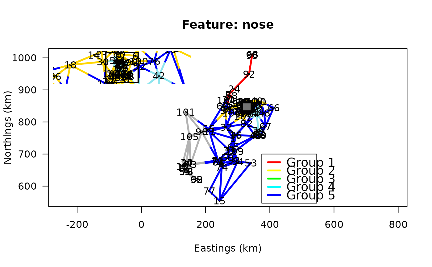
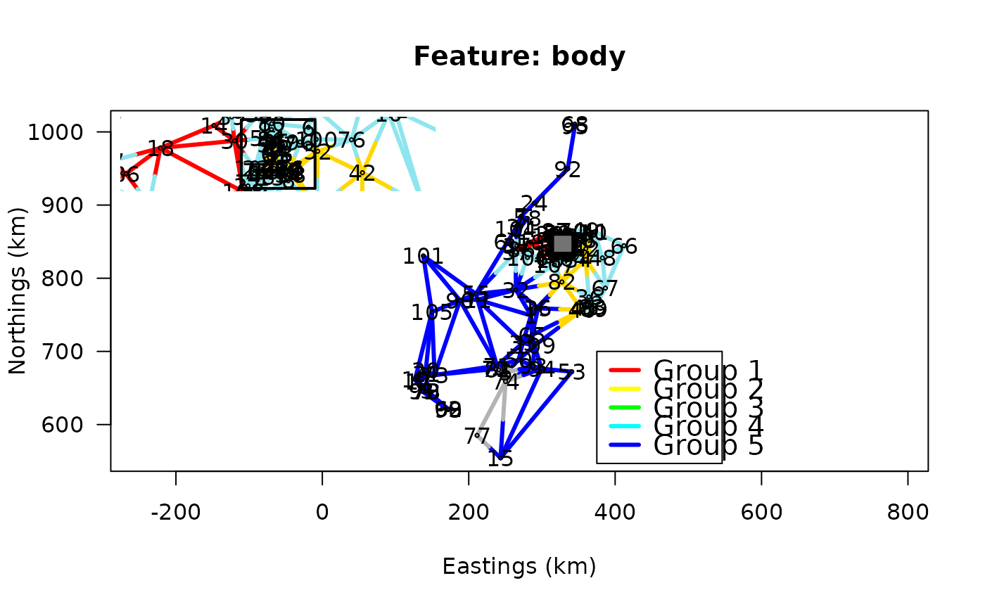
## Plot the clustering results on the map of Scotland for 5 groups.
## The inset map shows the Speyside distilleries in detail:
plotWhiskey("nose", 5L)

plotWhiskey("body", 5L)

plotWhiskey("palate", 5L)

plotWhiskey("finish", 5L)

plotWhiskey("norm", 5L)


## End of the Scotch Whiskey tasting data example

if (FALSE) { # \dontrun{

## Third example: Fish community composition along the Doubs River,
## France. The sequence is analyzed as a case of chronological
## clustering, substituting space for time.

if(require("ade4", quietly = TRUE)){
data(doubs, package="ade4")
Doubs.D <- dist.ldc(doubs$fish, method="hellinger")
grpWD2cst_fish <- constr.hclust(Doubs.D, method="ward.D2", chron=TRUE,
                                coords=as.matrix(doubs$xy))
plot(grpWD2cst_fish, k=5, las=1, xlab="Eastings (km)",
     ylab="Northings (km)", cex=3, lwd=3)

## Repeat the plot with other values of k (number of groups)

## End of the Doubs River fish assemblages example

## Example with 6 connected points, shown in Fig. 2 of Guénard & Legendre paper 

var = c(1.5, 0.2, 5.1, 3.0, 2.1, 1.4)
ex.Y = data.frame(var)

## Site coordinates, matrix xy
x.coo = c(-1, -2, -0.5, 0.5, 2, 1)
y.coo = c(-2, -1, 0, 0, 1, 2)
ex.xy = data.frame(x.coo, y.coo)

## Matrix of connecting edges E
from = c(1,1,2,3,4,3,4)
to = c(2,3,3,4,5,6,6)
ex.E = data.frame(from, to)

## Carry out constrained clustering analysis
test.out <-
    constr.hclust(
        dist(ex.Y),       # Response dissimilarity matrix
        method="ward.D2", # Clustering method
        links=ex.E,       # File of link edges (constraint) E
        coords=ex.xy      # File of geographic coordinates
    )

par(mfrow=c(1,2))
## Plot the map of the results for k = 3
plot(test.out, k=3)
## Plot the dendrogram
stats:::plot.hclust(test.out, hang=-1)
}

## Same example modified: disjoint clusters
## Same ex.Y and ex.xy as in the previous example
var = c(1.5, 0.2, 5.1, 3.0, 2.1, 1.4)
ex.Y = data.frame(var)

## Site coordinates, matrix xy
x.coo = c(-1, -2, -0.5, 0.5, 2, 1)
y.coo = c(-2, -1, 0, 0, 1, 2)
ex.xy = data.frame(x.coo, y.coo)

## Matrix of connecting edges E2
from = c(1,1,2,4,4)
to = c(2,3,3,5,6)
ex.E2 = data.frame(from, to)

## Carry out constrained clustering analysis
test.out2 <-
    constr.hclust(
        dist(ex.Y),       # Response dissimilarity matrix
        method="ward.D2", # Clustering method
        links=ex.E2,      # File of link edges (constraint) E
        coords=ex.xy      # File of geographic coordinates
    )
cutree(test.out2, k=2)

par(mfrow=c(1,2))
## Plot the map of the results for k = 3
plot(test.out2, k=3)
## Plot the dendrogram showing the disconnected groups
stats:::plot.hclust(test.out2, hang=-1)
axis(2,at=0:ceiling(max(test.out2$height,na.rm=TRUE)))

## End of the disjoint clusters example

} # }
## End of examples